How To Use The Choose Function In Google Sheets

The CHOOSE Function in Google Sheets lets you choose between different options.

It’s a lookup function, akin to a limited VLOOKUP rather than an alternative to the IF function.

It takes an index number and returns a value at that numbered position from the list of possible options.

Here’s a simple example:

which will output:

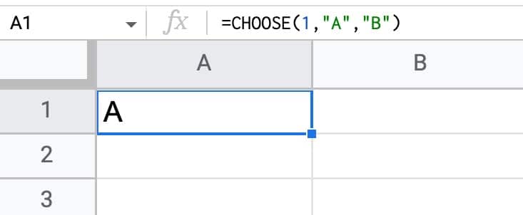
The first argument is the index number: 1.

Subsequent arguments are possible choices. The CHOOSE function returns the value at index position 1 in this case, i.e. “A”.

If I changed the index number to 2, the CHOOSE function would output “B”.

🔗 Get this example and others in the template at the bottom of this article.

CHOOSE Function Syntax

It takes a minimum of 2 arguments:

index

The first argument is required. It’s a number that indicates the position of the value you want to return from the list of possible values. It can be a number, a reference to a cell containing a number, or a nested function that generates a number.

choice1

The second argument is required and is the first possible value to return. Can be a value, reference to a cell, or a nested formula.

[choice2, ...]

Optional additional choices, up to a maximum of 29.

CHOOSE Function Notes

The index number must lie between 1 and the number of choices (up to a maximum of 29).

If the index number is negative, 0, or greater than the number of choices, a #NUM! error is returned.

When To Use The CHOOSE Function

The CHOOSE function can be used to lookup values when you have a limited number of them. It’s simpler and quicker than creating a VLOOKUP function, but doesn’t work so well with lots of values.

Here’s an example dataset showing students and their preferred activity: 1, 2, or 3.

The CHOOSE function quickly converts that to the activity name:

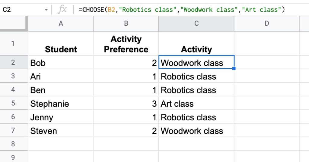
In this example, we referenced cell B2 as the input.

CHOOSE Formula Example

Suppose you have a dataset with a column of codes that represent the sale referral type.

CHOOSE converts the code to a description that we can understand:

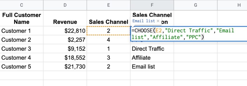
In this example, the CHOOSE formula is:

Again, the index number is in a cell (E2) rather than hard-coded into the CHOOSE formula.

Generating Random Data

Another great use case for CHOOSE is to generate random data.

For example, this formula will randomly select A, B, C, D, or E:

It uses the RANDBETWEEN function to generate a random number between 1 and 5 that then serves as the index number for CHOOSE.

This can be combined with other string formulas to generate fake data, e.g. this set of fictional invoice numbers:

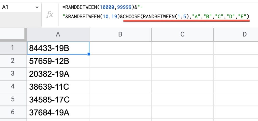
The formula to generate the data shown in this image is:

CHOOSE Function Template

Click here to open a view-only copy >>

Feel free to make a copy: File > Make a copy…

If you can’t access the template, it might be because of your organization’s Google Workspace settings.

In this case, right-click the link to open it in an Incognito window to view it.

It’s part of the Lookup family of functions in Google Sheets. You can read about it in the Google Documentation.