Have you ever wanted use the VLOOKUP function with multiple criteria?
For example, you may want to use first name and last name combined to search for a value using Vlookup.
In this post, you’ll see how to Vlookup multiple criteria in Google Sheets, with three different scenarios.
1. Vlookup Multiple Criteria into Single Column
In this case, we want to combine search criteria to use in the Vlookup formula. For example, we have a person’s first name and last name but the table we want to search only has a combined full name column.
The trick here is to nest a concatenation formula inside the Vlookup to combine the criteria prior to searching.
The formula for this Vlookup with multiple criteria is relatively straightforward:
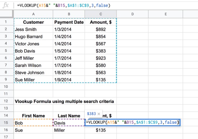
=VLOOKUP(A15&" "&B15,$A$1:$C$9,3,false)It’s a regular Vlookup formula, with concatenated values as the first argument. We need to combine first name and last name before searching for the full name in the table.
This part of the formula:
A15&" "&B15combines Bob in column A and Davis in column B into Bob Davis, which is the value we then search for in the table with Vlookup.
Want a copy of the example worksheet?
2. Vlookup Single Criteria into Multiple Columns with Helper Column
This scenario is the opposite way round to the first one. In other words we have a complete search term, but our search table has multiple columns that need to be searched.
For example, our search term is the full name of someone, but the search table has a column for first name and a column for last name. In this situation, we can’t perform a standard vlookup.
What we do is create a helper column in the search table, which combines the required columns to create a new search column. So we combine the first and last names to create a helper column containing the full name.
There are various concatenation formulas you could use to create a helper column, for example:
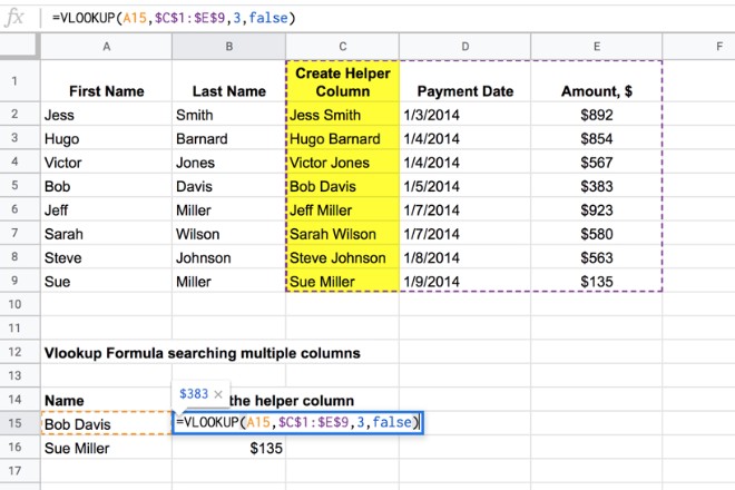
A2&" "&B2=JOIN(" ",A2:B2)=CONCATENATE(A2," ",B2)The helper column is shown in yellow in the image above.
Then it’s simply a standard Vlookup using this helper column as the search column.
For example, the formula in the image above uses the helper column C (yellow) as the search column:
=VLOOKUP(A15,$C$1:$E$9,3,false)Want a copy of the example worksheet?
3. Vlookup Single Criteria into Multiple Columns Dynamically with Array Formulas
This is exactly the same scenario as 2 above, but this time instead of creating a helper column directly in the table, we’ll use the Array Formula to do it all dynamically on the fly.
Breaking this down into steps:
3.1 Create Array of Criteria Columns
First we need to generate the array of full names using this formula:
=ArrayFormula($A$2:$A$9&" "&$B$2:$B$9)(This is an Array formula. You enter the ranges $A$2:$A$9&” “&$B$2:$B$9 and then hit Ctrl + Shift + Enter, or Cmd + Shift + Enter (Mac) to add the Array Formula designation.)
This is the result, generated by the single formula in cell B15:

3.2 Add the other columns from the original table
In this step we build the new search table by adding the other columns from the original table that we want to search, using this formula:
=ArrayFormula({$A$2:$A$9&" "&$B$2:$B$9,$C$2:$D$9})Here we’ve used array literals — the curly braces { … } — to combine arrays. Using a “,” between curly brace arrays treats them as columns next to each other, which is what we want in this case, as you can see in the image:
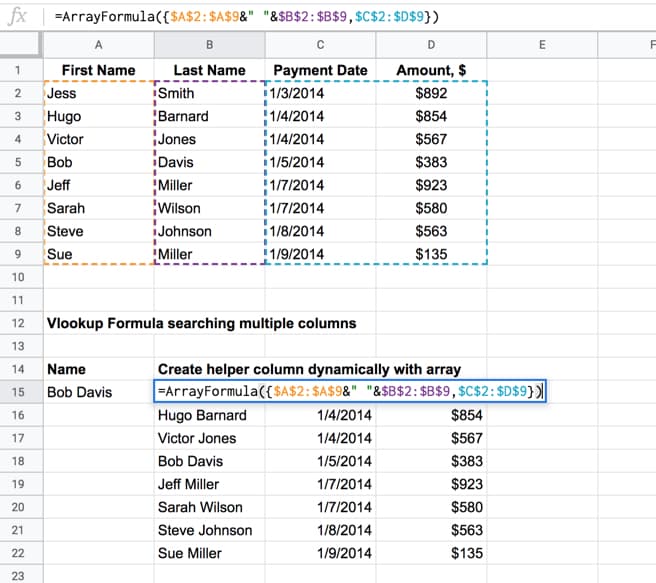
(Note 1: If we wanted arrays on top of each other, we use the “;” notation.)
(Note 2: For most European users, your syntax is a little different. Have a read of this post: Explaining syntax differences in your formulas due to your Google Sheets location.)
3.3 Perform the Vlookup
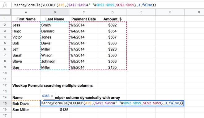
Now we have created a new table with the full name column, we simply use this as the range input in a standard vlookup, as shown in the first image of Section 3 above.
The formula to do this is:
=ArrayFormula(VLOOKUP(A15,{$A$2:$A$9&" "&$B$2:$B$9,$C$2:$D$9},3,false))Notice that the Array Formula wrapper stays on the outside of the whole formula.
Want a copy of the example worksheet?
Related Articles
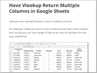 Have Vlookup Return Multiple Columns in Google Sheets
Have VLOOKUP return multiple columns in Google Sheets, with this quick and easy tutorial. Use an Array Formula wrapper to Vlookup multiple columns.
 How to do a Vlookup to the left in Google Sheets?
See how to create a new virtual table with an array, where the columns are switched, so the VLOOKUP can work on this new table.
 Vlookup in Google Sheets using wildcards for partial matches
See how to use a standard VLOOKUP formula with the wildcard asterisk character: *
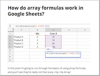 How do array formulas work in Google Sheets?
This post takes you through the basics of array formulas in Google Sheets, with example calculations and a worksheet you can copy.
Hi Ben, this is great but I want to do it the other way round. The range I am querying has the values in two different cells. Is that possible?
You should use index mach.
Hello. Thank you for the tutorial. I used your example 3 and modified it a bit to get it to do exactly what I need.
Now the next thing I need to do is import range, but I can’t get it to work. How would I add the import range to the example 3 below? Thanks.
=ArrayFormula(VLOOKUP(K27&” “&L27,{$K$11:$K$18&” “&$L$11:$L$18,$M$11:$O$18},{2,3,4},false))
so what if Bob Davis would have 2 payments and you would only want to see the newest payment?
You should put a condition. Or concatenate the total.or use Mach to select the value (equal,more than,less than).
Hi Ben, thank you for the tutorial.
I’d learn like to learn how the methods using vlookup and arrayformula would differ in effect. I’ve tried both and it seems to yield a similar effect. Thanks!
Thanks for sharing…. This seems really cumbersome. I really want to switch out to SQL database would make it so much easier. But I need to share with colleagues so using sheets is the best bet.
Is there an easier way? Should I use GAS?
Part 2 of my comment….
I just found the Filter function… it seems useful for having multiple criteria.
I have a question about this vlookup with two different condition Can you please help me to solve it? I have this spreadsheet https://docs.google.com/spreadsheets/d/1kZrbiaH3vUbnGNgZ9N34BiyHgvPdYUbLDcKRvuew8kA/edit?usp=sharing Please consider in the sheet “Ordini_di_lavorazione”, the formula in row n° 21 column L I wrote (and it’s wrong, i know…maybe also europe formula has different commas ….) =VLOOKUP((K21&V21;IMPORTRANGE(“https://docs.google.com/spreadsheets/d/1kZrbiaH3vUbnGNgZ9N34BiyHgvPdYUbLDcKRvuew8kA”;”2021-Schede_lavorazioni_IMPORT Epicollect!G:O”);6;FALSE)) What i would like is to import from the sheet “2021-Schede_lavorazioni_IMPORT Epicollect” the F9 because is in the ROW9 that i i found what i have in K21&V21…. I will be really greatfull for this Thank you!
Hello Ben Collins i want a Vlookup Formula for different result but reference is on one like; (A) have some Result but Reference is only A. Then who can we find out the result please .
thanks for the above, i have a peculiar issue, the data i need to look is based in two different rows so for example – i need to consider column “X” but only if it is based on the data of row “y”
column “PCS NO” but should pick up data from row “PCS Line” whereas column PCS No has 5 rows with various names such as “PCS Line” , “Sales Inv”, Pur Inv”……
Hi,
I Need help with this scenario.
I have two sheets Sheet A & Sheet B
Lets Say
Sheet A has 4 Columns (Data 1, Data 2, Data3, Data 4)
Sheet B has 6 Columns (Data 1, Data 2, Data3, Data 4, Data 5, Data 6)
Data 1 to 4 are same in both sheets
But the problem here is the order of the data is not same in both the sheets, like if some x data is in Row 1 in Sheet A, it will be in some 100th row in Sheet B.
How can we match the Data 1 to 4 on the sheet A and import the corresponding Data 5 & 6 in to Sheet A from Sheet B?
How about two vlookups searching for similar criteria on two sheets nested in an IFERROR. I can get it to work if the first vlookup returns a value, but it doesn’t and it has to search the second sheet I get “Not Applicable” statement in the cell instead of the value which I know is there.
what if we have to lookup dates in addition to texts.
like, same names are repeating with payment date and amounts, but we need an answer for date after X only.
hi i have three differents vendor name and price , i found the min value for those vendor, now i have to find the min vaule belongs which respective vendor in google sheet pls help on this