XLOOKUP Function in Google Sheets

The XLOOKUP function in Google Sheets is a new lookup function in Google Sheets that is more powerful and flexible than the older lookup functions like VLOOKUP or HLOOKUP.

XLOOKUP matches a search key in a lookup range and returns the value from a result range at that same position. If XLOOKUP does not find a match, you can specify a default value. You can control the match mode, like other lookup functions, and even control the search mode. More on that below, but first let’s see a simple example.

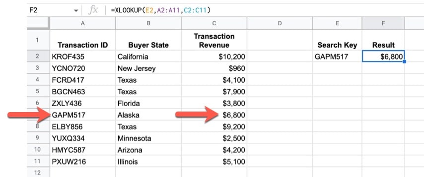
Here’s a simple XLOOKUP formula that looks for the search key in column A and returns a value from column C:

It looks like this in the Sheet:

🔗 Get this example and others in the template at the bottom of this article.

XLOOKUP Function Syntax

It takes a minimum of three and a maximum of six arguments:

search_key

The value you want to search for.

lookup_range

The range to search. It must be either a single column or a single row.

result_range

The range to consider for the result. The return value is taken from the position of the matched value in the lookup array if the search key is found. The result range must match the dimensions of the lookup range.

[missing_value]

The fallback value to return if no match exists. This is an optional argument and if it is omitted, an error is returned if no match exists.

[match_mode]

This optional argument lets you specify what match mode to use. If unspecified, an exact match is used.

The options are:

Option	Match Mode Behavior
0	Exact match search
1	Exact match or next value that is bigger than the search key
-1	Exact match or next value that is lower than the search key
2	Wildcard match

[search_mode]

This optional argument lets you specify what search mode to use. If it is omitted, XLOOKUP defaults to searching the lookup range from the first entry to the last entry.

The different search options are:

Option	Search Mode Behavior
1	Search from the first entry to the last one
-1	Search from the last entry to the first
2	Search through the range using binary search and assuming the range is sorted in ascending order
-2	Search through the range using binary search and assuming the range is sorted in descending order

XLOOKUP Function Notes

• The lookup range can only be either a single row or a single column. It cannot be an array with multiple rows and columns.
• The result range must be compatible with the size of the lookup range. For example, if the lookup range is a column of data with 10 rows and 1 column, then the result range must also have 10 rows (though it can have more than 1 column).

XLOOKUP Function Examples

Let’s see some more examples of the XLOOKUP function in Google Sheets.

Example 1: Basic Exact Match

If you omit the optional match mode argument, the XLOOKUP function will perform an exact match.

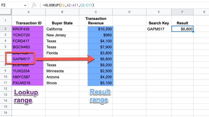
I.e. when you write it with only the first three arguments, a search key, a lookup range, and a result range, then it will look for an exact match. We saw this in the example at the top of this page:

Which works like this in the Sheet:

Example 2: Missing Value

Now, we can specify a fallback value if no match is found. This is done with the fourth (optional) argument, e.g.

In our Sheet:

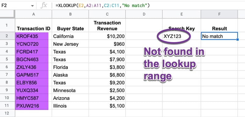
In this case, the search key “XYZ123” is not found in the lookup array (column A) so the XLOOKUP function returns the fallback missing value, which we set to “No match”.

Example 3: XLOOKUP Function Left

Another benefit with the XLOOKUP function is that the lookup range does not have to be to the left of the result range, which is the case with the VLOOKUP (though there is a complicated workaround with array literals).

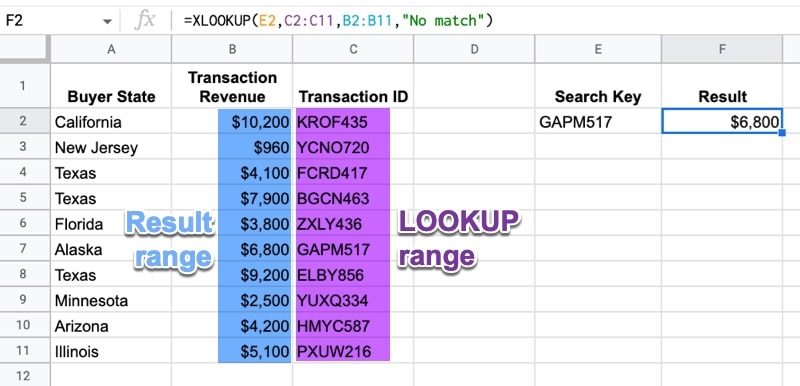
The formula does not change, but this time the result range is positioned to the left of our lookup range:

As you can see, it works equally well in our Sheet:

Example 4: Approximate Match

The fifth argument of the XLOOKUP function determines the matching mode. If it is omitted or set to 0, then an exact match is performed.

However, there are situations where the approximate matching option works really well.

Consider the case when our search key falls between two values in the lookup range. It’s not an exact match, but we might still want to return a result to say that it’s lower than X, or higher than Y.

For example, consider this bank savings scenario:

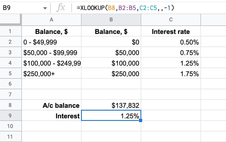
The XLOOKUP formula for this example is:

Notice the -1 as the final argument, which tells the function to look for an exact match and if it doesn’t find one, to return the value that is lower in the array.

In this example, it doesn’t find the $137,832 exactly, so it looks at the lower value in the array, i.e. $100,000. This is in position 3 of the lookup array, so it returns the value from the 3rd position of the results array, i.e. 1.25%.

One final thing to mention with this example, notice how the fourth argument is blank. This is where we can specify a “missing value” for when no match is found. However, it’s not required here because we’re using an approximate match anyway.

Example 5: Wildcard Match

XLOOKUP in Google Sheets supports three wildcards, *, ?, and ~.

The star * matches zero or more characters.

The question mark ? matches exactly one character.

The tilde ~ is an escape character that lets you search for a * or ?, instead of using them as wildcards.

Let’s see an example that uses a surname to find the full name:

And another example that uses a surname to return transaction revenue from that row:

Both formulas are seen in the following image, with the first one in cell B17 and the second in cell B18:

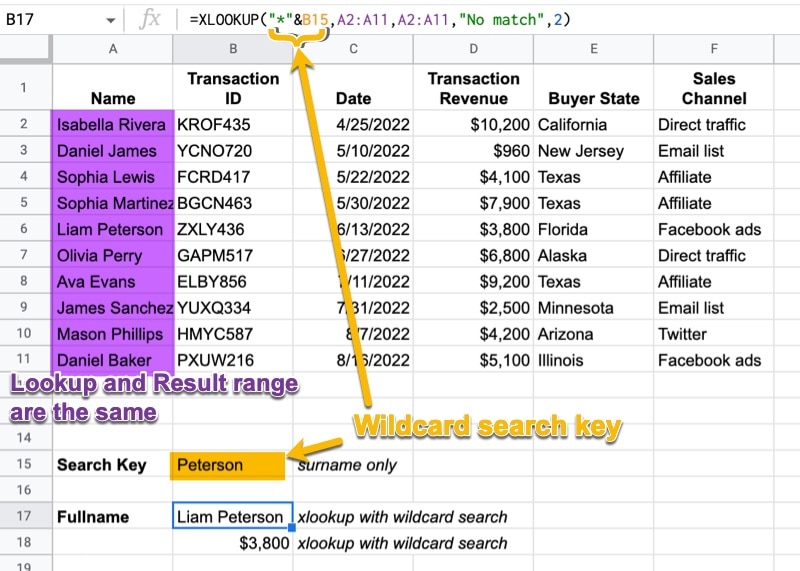
There are two important things to notice with this formula:

1) The search key is “Peterson”, but to use it in the XLOOKUP function, we first add the wildcard star character that matches anything before the “Peterson”:

I.e. *Peterson

Note, if there were multiple “Peterson” in this dataset this could cause an issue. In this case, you might want to try using the QUERY function or the FILTER function to return all the “Peterson” results.

2) The match mode in the fifth argument is set to 2, which indicates that this is a wildcard search.

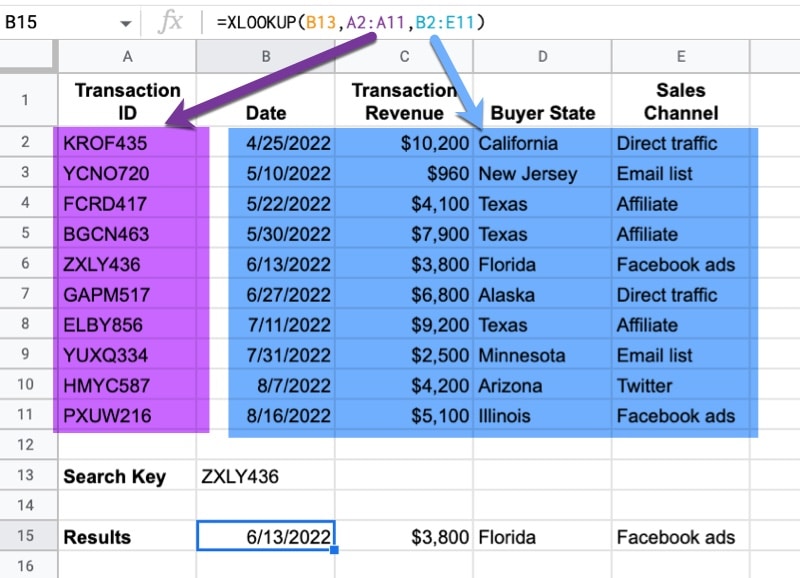
Example 6: Return Multiple Results

The XLOOKUP function can return multiple results for a single match, not just a single result like a VLOOKUP (although there is a workaround for VLOOKUP to return multiple columns).

XLOOKUP returns multiple results by specifying a result range with multiple columns (or rows if you’re doing a horizontal lookup).

The formula is:

This gives the result:

Example 7: Different Search Mode

The final argument lets you change the search method used. The default is to search from top to bottom of your range, but you can change this to search from the bottom to the top if that makes sense.

The XLOOKUP can also perform super quick binary searches, but this requires your data to be sorted correctly to avoid incorrect results.

XLOOKUP Function Template

Click here to open a view-only copy >>

Feel free to make a copy: File > Make a copy…

If you can’t access the template, it might be because of your organization’s Google Workspace settings.

In this case, right-click the link to open it in an Incognito window to view it.

It’s part of the Lookup family of functions in Google Sheets. You can read about it in the Google Documentation.