How To Highlight The Top 5 Values In Google Sheets With Formulas

In this post, you’ll learn how to find and highlight the top 5 values in Google Sheets.

For all the examples that follow, we’ll use this dataset, which is available in the downloadable template at the end of this post:

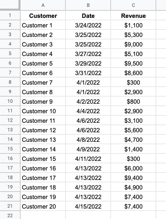
We’ll see how to highlight the rows with the top 5 values, as well as how to extract those values using SORTN.

How To Highlight The Top 5 Values In Google Sheets

Method 1: Use the LARGE Function

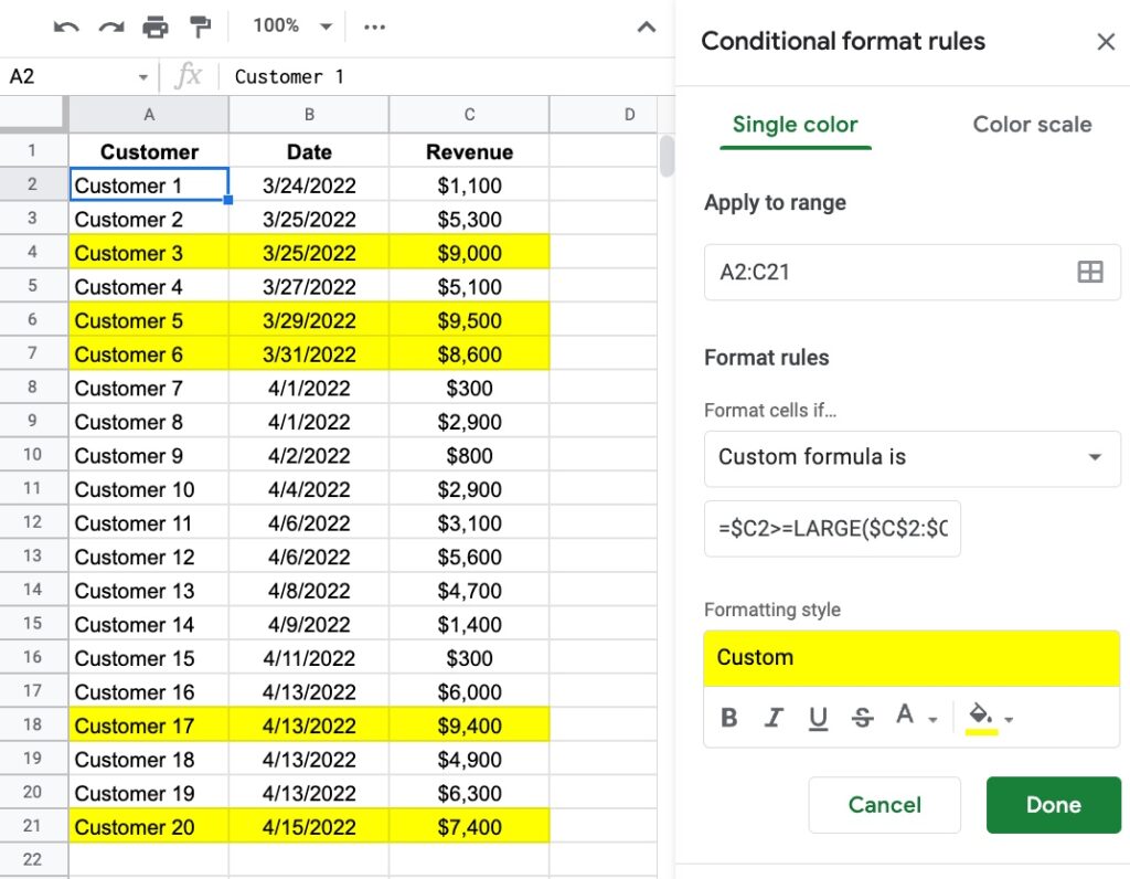
Highlight your data range, in this case, A2:C21 (omitting the header row).

Then go to the menu: Format > Conditional formatting

Under Format rules, select Custom formula is

Enter this formula (explained below):

Set your formatting styles like the yellow background color shown in this example.

Your conditional formatting sidebar should look like this:

Boom!

The conditional formatting will highlight the top 5 values in your table.

How does this formula work?

The LARGE function returns the nth largest element from a dataset.

In this example, it returns the 5th largest value from column C of our data:

(If you want the top 10 values, simply change the 5 to a 10.)

Notice the $ signs around the range are required for the conditional formatting. They turn the range into an absolute reference so it stays locked on column C.

This part of the formula (in red):

tests each row to see if it’s larger than or equal to this 5th largest value.

Notice the $ in front of the first C, but not in front of the 2, i.e. $C2 not $C$2. This is crucial to apply conditional formatting across the whole row.

Method 2: Use the RANK Function

Follow the steps above, but use the RANK function as the basis for the custom formula instead:

How does this formula work?

The RANK function returns the position of a value within a set of values.

In this example, the RANK function returns the rank of each value in column C:

As earlier, note the position of the $ signs around the cell references as these are crucial when we create the conditional formatting rule.

The full formula then checks if it’s less than or equal to 5.

(If you want the top 10 values, simply change the 5 to a 10.)

If the value satisfies this criterion, then the conditional formatting is applied to the whole row.

Now, suppose you want to return the top 5 rows, rather than just highlight them, how would you do that?

How To Find The Top 5 Values In Google Sheets With The SORTN Function

The SORTN function sorts your data and returns the first N items.

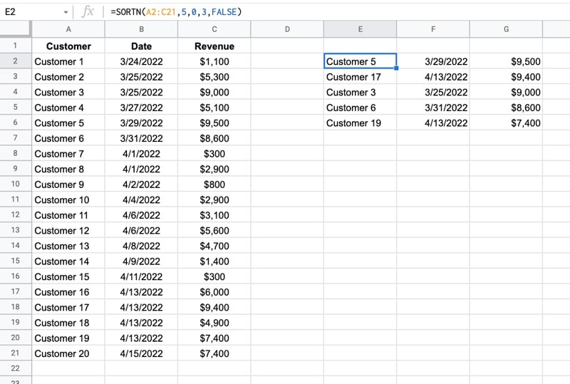
This formula will return the top 5 rows from the data:

It sorts the data from high to low and returns only the first five values.

The SORTN function has a lot of options.

From left to right, the arguments inside the formula are:

$A$2:$C$21 is the range to sort.

5 is how many results to return. If you want the top 10 values, simply change the 5 to a 10.

0 ensures the SORTN returns only 5 values. You can specify other options to deal with ties.

3 is the number of the column to sort, which represents column C in this example.

FALSE sorts in descending order, high to low. TRUE sorts ascending.

Highlight The Top 5 Values In Google Sheets Template

Click here to open a view-only copy >>

Feel free to make a copy: File > Make a copy

If you can’t access the template, it might be because of your organization’s Google Workspace settings. If you right-click the link and open it in an Incognito window you’ll be able to see it.