 💡 Learn more
Learn more about working with Lambda Functions, Named Functions, and X-Functions in the FREE Lambda Functions 10-Day Challenge course
The XMATCH function in Google Sheets is a new lookup function in Google Sheets that finds the relative position of a search term within an array or range. It’s an evolution of the original MATCH function.
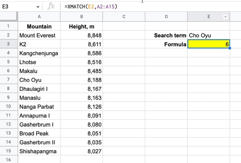
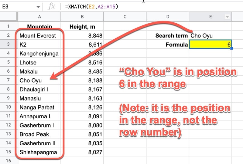
Here’s a simple XMATCH function that finds the position of the search term “Cho Oyu” in the list of the highest mountains in the world:
=XMATCH(E2,A2:A15)In the Sheet:
And here’s how it works:
It looks for the search term from cell E2 (“Cho Oyu”) in the range A2:A15, then returns the position of the search text within this range. Note that the result is relative to the range, irrespective of the row number.
Notice how, unlike a regular MATCH function, you don’t have to specify the “0” search type for an exact match. It chooses the exact match, which is by far the most common use case, by default (in contrast to the MATCH function where you have to add the 0 to explicitly confirm exact matching). More on the search types below.
🔗 Get this example and others in the template at the bottom of this article.
XMATCH Function Syntax
=XMATCH(search_key, lookup_range, [match_mode], [search_mode])It takes 4 arguments in total, the last 2 being optional:
search_key
This is the value you want to search for.
lookup_range
The range to search. It must be a single row or column.
[match_mode]
This optional argument lets you specify what match mode to use. If unspecified, an exact match is used.
The options are:
| Option | Match Mode Behavior |
| 0 | Exact match search |
| 1 | Exact match or next value that is bigger than the search key |
| -1 | Exact match or next value that is lower than the search key |
| 2 | Wildcard match |
[search_mode]
This optional argument lets you specify what search mode to use. If it is omitted, XMATCH defaults to searching the lookup range from the first entry to the last entry.
The different search options are:
| Option | Search Mode Behavior |
| 1 | Search from the first entry to the last one |
| -1 | Search from the last entry to the first |
| 2 | Search through the range using binary search and assuming the range is sorted in ascending order |
| -2 | Search through the range using binary search and assuming the range is sorted in descending order |
XMATCH Function Notes
- The lookup range can only be either a single row or a single column. It cannot be an array with multiple rows AND columns.
- If an exact search mode is used but no match is found, the XMATCH function returns a #N/A error.
XMATCH Function Examples
For the following examples, let’s use this dataset of the highest mountains in the world:
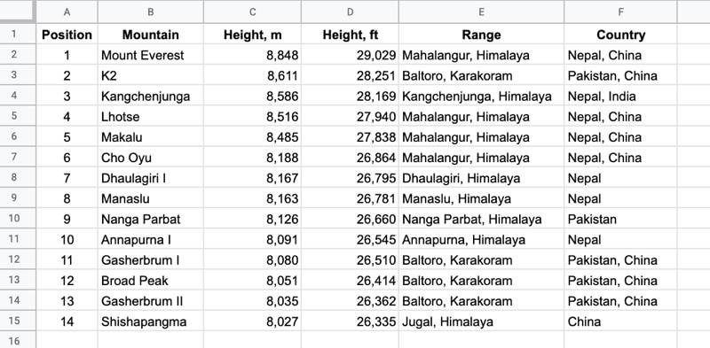
(This is available in the template, linked at the bottom of this article.)
Example 1: Basic Exact Match
If you omit the optional match mode argument, or set it to 0, the XMATCH function will perform an exact match. This is the example we saw at the top of this blog post:
Example 2: Next Value XMATCH
The third argument of the XMATCH function determines the matching mode. As you saw above, in example 1, if it is omitted or set to 0, then an exact match is performed.
However, if we set it to 1 or -1, then the approximate matching mode is used.
Consider the case when our search key falls between two values in the lookup range. It’s not an exact match, but we might still want to return a result that is higher or lower than it.
Setting the match mode to 1 will find an exact match (if it exists) or the next value that is bigger than the search key.
Setting to -1 will find an exact match (if it exists) or the next value that is lower than the search key.
Consider this example:
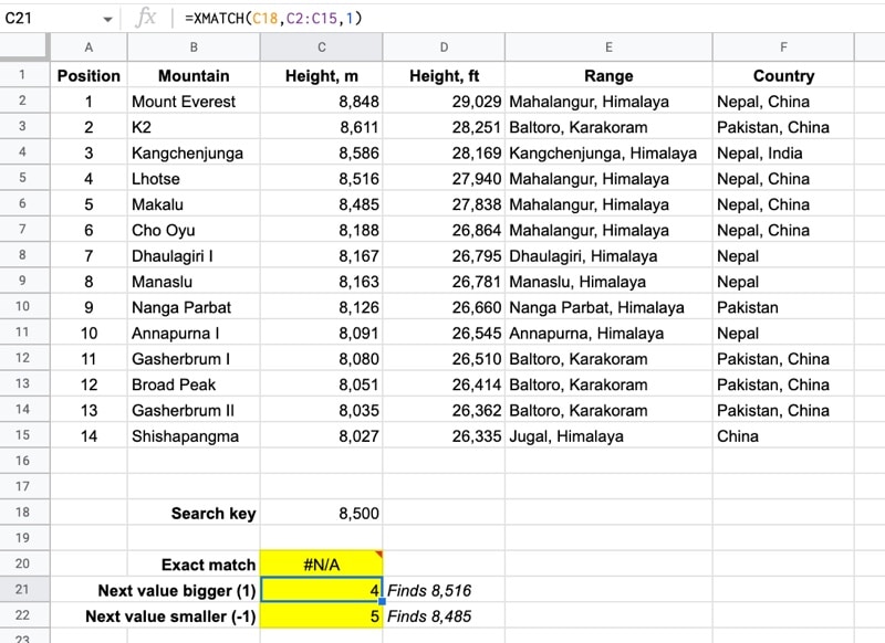
The search term is 8,500 which does not occur in the search range (C2:C15).
The formula to find the next value that is bigger than the search term (i.e. > 8,500) is:
=XMATCH(C18,C2:C15,1)Since 8,500 is not found exactly, it finds the next largest value (8,516) and returns the relative position of that item, i.e. position 4 in this example.
The formula to find the next value that is lower than the search term (i.e. < 8,500) is:
=XMATCH(C18,C2:C15,-1)In this example, it doesn’t find the 8,500 exactly, so it looks at the lower value in the array, i.e. 8,485, which is in position 5 of the lookup range.
Example 3: Wildcard XMATCH
XMATCH in Google Sheets supports three wildcards, *, ?, and ~.
The star * matches zero or more characters.
The question mark ? matches exactly one character.
The tilde ~ is an escape character that lets you search for a * or ?, instead of using them as wildcards.
Let’s see an example that uses a partial name to find the position of the full name.
The search term from cell C18 is “Annapurna”, to which we add a “*” wildcard character. This tells the XMATCH function to match anything that begins with “Annapurna”.
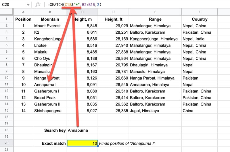
The formula is:
=XMATCH(C18&"*",B2:B15,2)It matches against “Annapurna I” and returns the position of that item, giving us the answer 10.
Example 4: Search Mode In XMATCH
The fourth argument, which is optional, determines the search mode of the XMATCH function.
If omitted, the default is mode 1, which searches top-down, from the first entry to the last.
However, you can choose to search from the bottom up, by setting the value to -1.
Let’s see an example of the difference in searching from the top-down versus bottom-up. Here, we search for the term “Pakistan, China” in the country column:
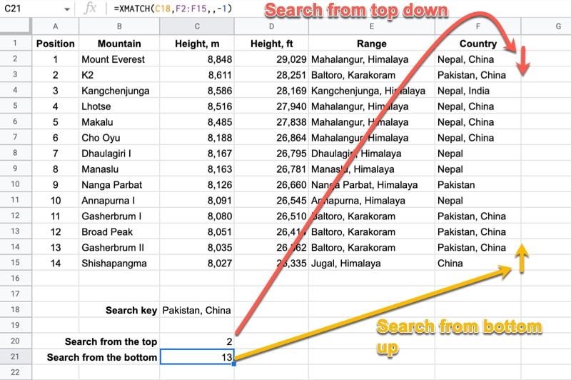
Search mode 1 finds the first instance, in position 2. The formula is:
=XMATCH(C18,F2:F15,,1)The search mode -1 finds the first instance starting at the bottom of the dataset and working up, and returns position 13 as the answer.
The formula is:
=XMATCH(C18,F2:F15,,-1)With both of these formulas, notice we left the third argument blank, which means it defaults to an exact match behavior.
Additionally, you can choose to use a binary search method and set the search mode to 2 (top-down) or -2 (bottom-up), designed to be faster when searching over really large datasets. This requires the data to be in ascending or descending order respectively.
Example 5: INDEX + XMATCH
The XMATCH function pairs extremely well with the INDEX function, to perform flexible, robust lookups.
XMATCH searches for a value and returns the position. Then INDEX is used to return the value in another cell in the same relative position of a range.
Let’s see an example:
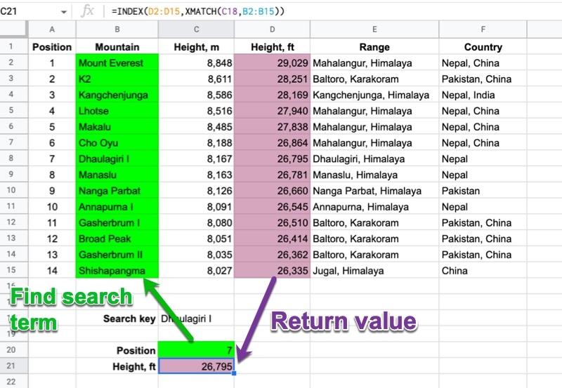
This formula finds the position of the search term “Dhaulagiri I”:
=XMATCH(C18,B2:B15)The answer is 7.
We then nest this XMATCH function inside the INDEX function (an example of using the Onion framework for formulas):
=INDEX(D2:D15,XMATCH(C18,B2:B15))This formula returns the value from column D (the height in ft.) in position 7, i.e. the height that corresponds to the position of “Dhaulagiri I”. The result is 26,795 ft.
XMATCH Function Template
🔗 Click here to open a view-only copy >>
Feel free to make a copy: File > Make a copy…
If you can’t access the template, it might be because of your organization’s Google Workspace settings.
In this case, right-click the link to open it in an Incognito window to view it.
The XMATCH function is also covered in the Day 9 lesson of my free Lambda Functions 10-Day Challenge course.
It’s part of the Lookup family of functions in Google Sheets. You can read about it in the Google Documentation.