Welcome to the Sheets Insiders newsletter #8, your exclusive, members-only publication.
You can see the full archives here.
This week, we’re continuing with the theme of what I call the “modern analytical functions” in Google Sheets.
Specifically, we’ll be using HSTACK, VSTACK, BYROW, LAMBDA, and LET.
These functions let us solve complex problems and create sophisticated formulas without needing code. And, they are often more readable than the equivalent formulas written with older methods.
This tutorial was covered in a live session earlier today. The replay is available below.
Live Session Replay
Template

Download the Modern Analytic Functions Template
Click on “Use Template” in the top right corner to make your own copy.
There is no Apps Script with this template.
Example 1: VSTACK Tables
Consider these two Tables, called “Batch1” and “Batch2”, that we want to combine into a single dataset:
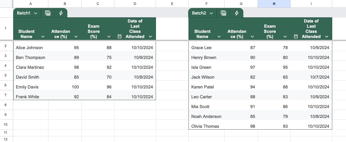
Conveniently, they have identical columns, so we’re able to stack them on top of each other.
But, suppose the Tables were larger and it was impossible to compare the headings at a glance.
We can use this lovely formula to verify that the header rows match:
=ARRAYFORMULA(AND(A1:D1 = F1:I1))
where A1:D1 is the range of data for headers in Table 1 and F1:I1 the same for Table 2.
Soon, with the new improvements to Table referencing, we’ll soon be able to do this:
=ArrayFormula(AND(Table1[#HEADERS]=Table2[#HEADERS]))
Then this formula will stack the Tables on top of each other:
=VSTACK(Batch1[#ALL],Batch2)
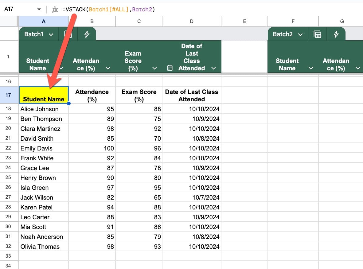
We include the header row from the first Table by using the [#ALL] designation.
(Learn more about Table referencing here.)
Example 2: Join Data Tables
Consider these two data Tables, called “Table1” and “Table2”, which have the same individuals but different data points:
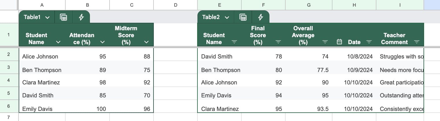
We want to combine (or “join”) these Tables so that each individual has the complete set of data points about them in a single Table.
It looks like a candidate for HSTACK (horizontal stack) but here’s the problem. The HSTACK does not match the rows correctly, it simply stacks the Tables next to each other.
That means unless your rows are perfectly lined up, you’ll get data on the wrong row, which will be a HUGE problem.
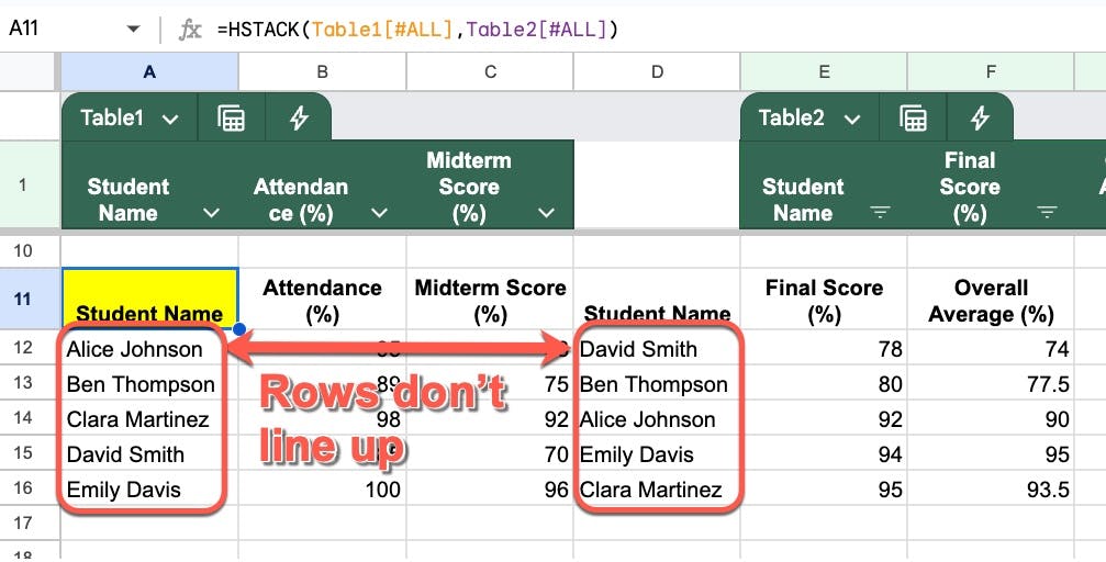
Much better in this scenario to use one of the other new functions, XLOOKUP, to correctly join the data:
=XLOOKUP(A19,Table2[Student Name],Table2)
Now, the correct data will be matched so that the rows display data for only that student name.
Example 3: Formula Headers
Consider this Table, called “example3”:
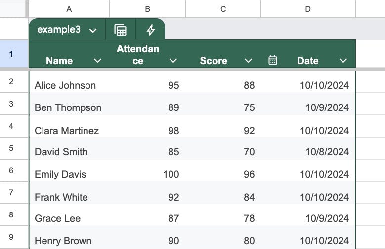
This FILTER function returns all the data with a score less than 80%:
=FILTER(example3,example3[Score]<80)
We can add a header row using formulas as follows:
=VSTACK(A1:D1, FILTER(example3,example3[Score]<80))
And soon, with the new Table referencing update, we’ll be able to grab the Table header row so our formula looks like this:
=VSTACK(example3[#HEADERS], FILTER(example3,example3[Score]<80))

Example 4: BYROW Date Formula
Consider this list of dates:

We want to separate out the day, month, and year.
There are two pieces to the puzzle:
- We can use an array formula to work on all the rows with a single formula.
- We can use HSTACK to deal with all the columns at once.
There’s nothing wrong with using an old-school ArrayFormula approach, but today we’re talking about modern functions. So let me introduce BYROW and LAMBDA.
BYROW
Here’s the BYROW formula that will extract the day number for each row:
=BYROW(A2:A11, LAMBDA( r , DAY(r)))
Breaking this down:
- The BYROW input is A2:A11, which is the range of dates
- LAMBDA is a special function where we define what happens to each row (i.e. each value in the input array)
- First is “r” and this is a placeholder for each row.
- Second is the action “DAY(r)” which in this case takes the value r and applies the function DAY to calculate the day number.
So, first it takes the value from A2, which is the date “11/20/2024” and applies the formula DAY(). This gives the output 20, which goes into the first cell of the output.
Then BYROW takes the second value (the date “12/15/2024” from cell A3) and applies DAY. The result is 15.
And so on and so forth until all the rows from the input range are complete.
HSTACK
We use HSTACK to combine all the operations:
=HSTACK( DAY(A2) , MONTH(A2) , YEAR(A2) )
Combined
Now we can combine the BYROW and HSTACK, as follows:
=BYROW( A2:A11 , LAMBDA( r , HSTACK( DAY(r) , MONTH(r) , YEAR(r) )))
We replaced the DAY(r) with the full HSTACK version HSTACK( DAY(r) , MONTH(r) , YEAR(r) as the operation to be done on each row.
In our Sheet:
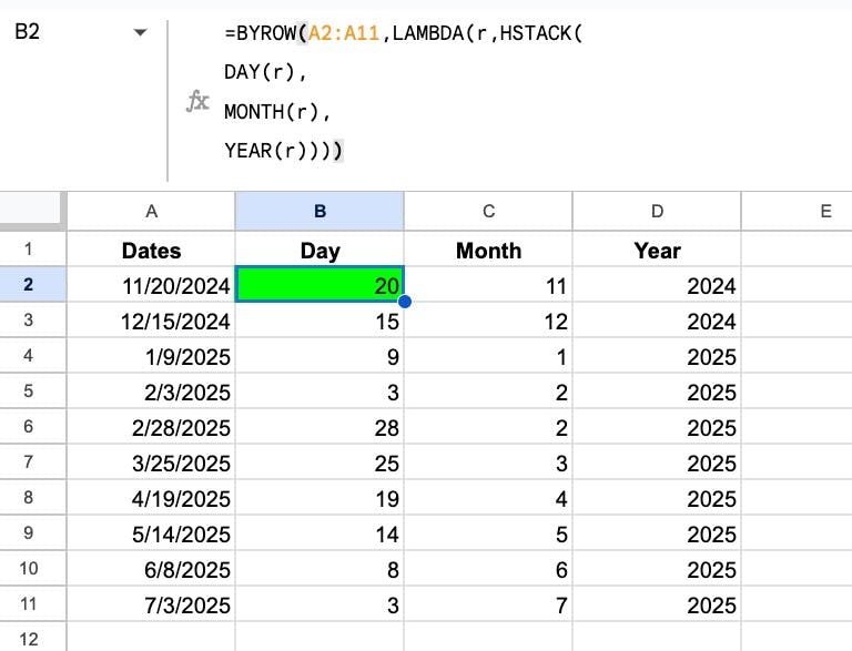
Nice!