Status arrows are little up or down symbols added to data that make it quick and easy to understand what’s happening. They’re a useful way to highlight changes in your data.
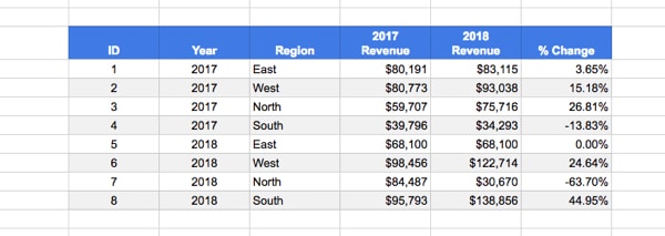
Consider the following sales data which has a % change column:
Now take a look at the same data with colors and arrows added to call out the % change column:
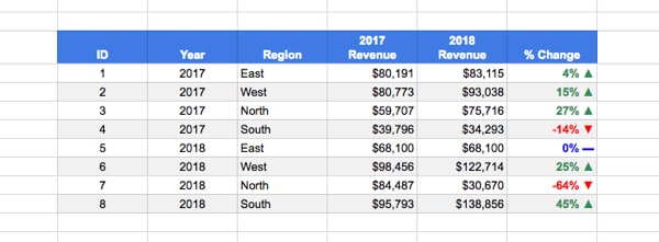
It’s significantly easier/quicker to read and absorb that information.
How to Add Status Arrows
Hidden in the Custom Number Format of Google Sheets is a conditional formatting option for setting different formats for numbers greater than 0, equal to 0, or less than zero. This can be used to show the up or down status arrows.
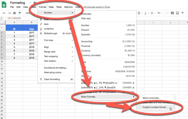
Step 1. Highlight the % column and go to the custom number formatting menu:
Step 2. Copy and paste this custom number format rule into the Custom number formats popup:
[color50]0% ▲;[color3]-0% ▼;[blue]0% ▬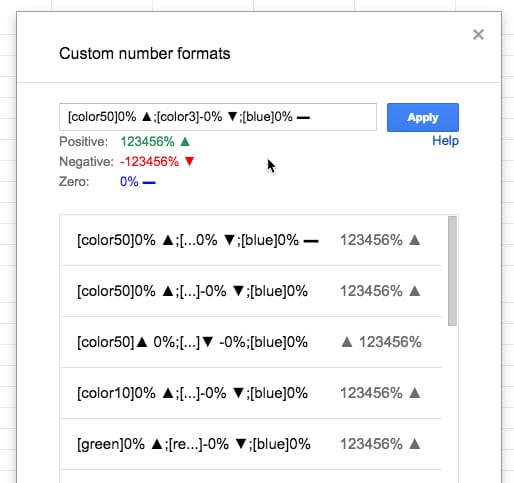
What you’re doing is specifying a number format for positive numbers first, then negative numbers and then zero values, each separated by a semi-colon.
The square brackets to specify the color you want e.g. [color50] for green. See the full list of colors here: Custom Number Format Color Palette Reference Table
The cells in the data are still numbers even though the status arrows are showing. The arrows are a visual layer on top of the number.
Great post. Is there a list of what colors the [colorX] corresponds to?
Full list of color codes here: https://www.benlcollins.com/spreadsheets/custom-number-format-color-palette-reference-table/