This Formula Challenge originally appeared as part of Google Sheets Tip #52, my weekly newsletter, on 27 May 2019.
Sign up here so you don’t miss out on future Formula Challenges:
Find all the Formula Challenges archived here.
Your Challenge
Start with this small data table in your Google Sheet:
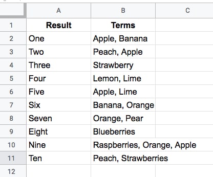
Your challenge is to create a single-cell formula that takes a string of search Terms and returns all the Results that have at least one matching term in the Terms column.
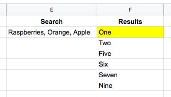
For example, this search (in cell E2 say)
Raspberries, Orange, Apple
would return the results (in cell F2 say):
One
Two
Five
Six
Seven
Nine
like this (where the yellow is your formula):
Check out the ready-made Formula Challenge template.
The Solution
Solution One: Using the FILTER function
=FILTER(A2:A11,REGEXMATCH(B2:B11,JOIN("|",SPLIT(E2,", "))))or even:
=FILTER(A2:A11,REGEXMATCH(B2:B11,SUBSTITUTE(E2,", ","|")))These elegant solutions were also the shortest solutions submitted.
There were a lot of similar entries that had an ArrayFormula function inside the Filter, but this is not required since the Filter function will output an array automatically.
How does this formula work?
Let’s begin in the middle and rebuild the formula in steps:
=SPLIT(E2,", ")The SPLIT function outputs the three fruits from cell E2 into separate cells:
Raspberries Orange Apple
Next, join them back together with the pipe “|” delimiter with
=JOIN("|",SPLIT(E2,", "))so the output is now:
Raspberries|Orange|Apple
Then bring the power of regular expression formulas in Google Sheets to the table, to match the data in column B. The pipe character means “OR” in regular expressions, so this formula will match Raspberries OR Orange OR Apple in column B:
=REGEXMATCH(B2:B11,JOIN("|",SPLIT(E2,", ")))On its own, this formula will return a #VALUE! error message. (Wrap this with the ArrayFormula function if you want to see what the array of TRUE and FALSE values looks like.)
However, when we put this inside of a FILTER function, the correct array value is passed in:
=FILTER(A2:A11,REGEXMATCH(B2:B11,JOIN("|",SPLIT(E2,", "))))and returns the desired output. Kaboom!
Solution Two: Using the QUERY function
=QUERY(A2:B11,"select A where B contains '"&JOIN("' or B contains '",SPLIT(E2,", "))&"'")As with solution one, there is no requirement to use an ArrayFormula anywhere. Impressive!
This formula takes a different approach to solution one and uses the QUERY function to filter the rows of data.
The heart of the formula is similar though, splitting out the input terms into an array, then recombining them to use as filter conditions.
=JOIN("' or B contains '",SPLIT(E2,", ",0))which outputs a clause ready to insert into your query function, viz:
Raspberries' or B contains 'Orange' or B contains 'Apple
The QUERY function uses a pseudo-SQL language to parse your data. It returns rows from column A, whenever column B contains Raspberries OR Orange OR Apple.
Wonderful!
Click here to open a read-only version of the solution template (File > Copy to make your own editable copy).
I hope you enjoyed this challenge and learnt something from it. I really enjoyed reading all the submissions and definitely learnt some new tricks myself.
SPLIT function caveats
There are two dangers with the Split function which are important to keep in mind when using it (thanks to Christopher D. for pointing these out to me).
Caveat 1
The SPLIT function uses all of the characters you provide in the input.
So
=SPLIT("First sentence, Second sentence", ", ")will split into FOUR parts, not two, because the comma and the space are used as delimiters. The output will therefore be:
First sentence Second sentence
across four cells.
Caveat 2
Datatypes may change when they are split, viz:
=SPLIT("Lisa, 01",",")gives an output of
Lisa 1
where the string has been converted into a number, namely 1.