Google Sheets REGEX Formulas

This post explores the Google Sheets REGEX formulas with a series of examples to illustrate how they work.

Regular expressions, or REGEX for short, are tools for solving problems with text strings. They work by matching patterns.

You use REGEX to solve problems like finding names or telephone numbers in data, validating email addresses, extracting URLs, renaming filenames containing the word “Application” etc.

They have a reputation for being hard, but once you learn a few basic rules and understand how they work you can use them effectively.

There are three Google Sheets REGEX formulas: REGEXMATCH, REGEXEXTRACT, and REGEXREPLACE.

Each has a specific job:

• REGEXMATCH will confirm whether it finds the pattern in the text.

• REGEXEXTRACT will extract text that matches the pattern.

• REGEXREPLACE will replace text that matches the pattern.

Let’s understand them with a series of examples.

Table Of Contents

• Example 1: Google Sheets REGEXMATCH
• Example 2: Google Sheets REGEXEXTRACT
• Example 3: Google Sheets REGEXREPLACE
• Example 4: Use REGEXEXTRACT And VALUE To Extract Numbers From Text
• Example 5: Check Telephone Numbers With REGEXMATCH
• Example 6: Reorder Name Strings With REGEXREPLACE
• SOLUTION From Example 1 Question
• Learn More

Example 1: Google Sheets REGEX Formula REGEXMATCH

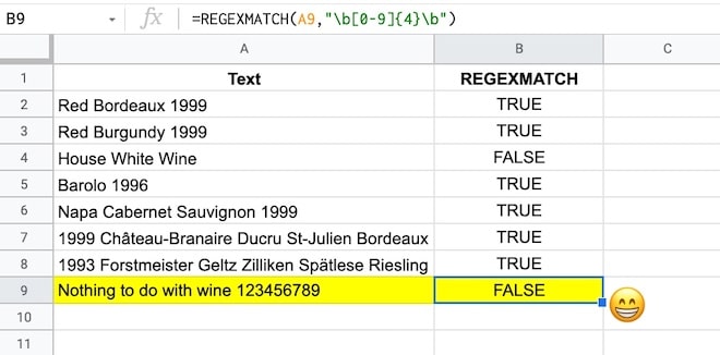
The REGEXMATCH function returns a TRUE if it matches the pattern you provide anywhere in the text and FALSE if there are no matches in the text.

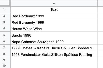
For example, suppose we have this dataset of vintage wines, where each row has a mix of text and/or numbers:

Let’s create a simple REGEXMATCH to test whether a cell contains a number, i.e. the year vintage is given.

In cell A2, add this formula:

This will give a TRUE output if it finds a number in the string, or FALSE if there are no numbers.

matches any number from 0 to 9 in the input string.

So, provided there is one number in the input string, this pattern will give us a match:

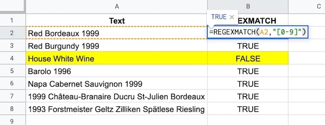
See how the text without any numbers “House white wine” gives a FALSE output because there is no match.

Important Note

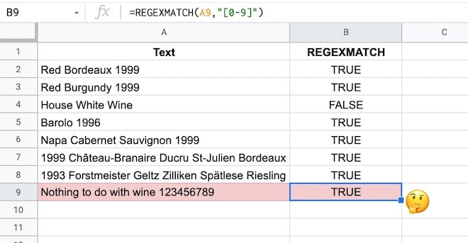
This pattern matches a single number. It doesn’t care what else might be in the cell.

For example, it returns TRUE for a meaningless string containing numbers, which is probably not the behavior you’re looking for in this case.

By the end of this tutorial, you’ll understand enough to know how to fix this yourself.

(For the solution, see the formula at the end of this tutorial.)

Example 2: Google Sheets REGEX Formula REGEXEXTRACT

Using the same wine dataset as above, we want to create a new column in our dataset with the vintages, i.e. a column with the year only.

This is a perfect example of when to use a Google Sheets REGEX formula. We’ll create a regular expression pattern to match any numbers and then use REGEXEXTRACT to extract them.

As with everything in spreadsheets, there are multiple REGEX patterns that could solve this.

We saw this pattern above:

but we can also use the named character class for digits:

This matches any digits (i.e. numbers 0 to 9).

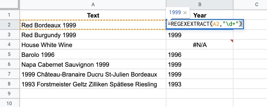
So the REGEXEXTRACT formula to extract the year looks like this:

or

Then

means get one or more.

Both formulas return a result of “1999” because the text in A2 is “Red Bordeaux 1999”.

If no numbers are found, the formula returns a #N/A error.

Two Important Notes

Note 1:

The REGEX formulas require text inputs and they give you text outputs back. So the 1999 output above is formatted as text. To convert to a number you need to wrap the result with a VALUE function. See Example 4 below for more details.

Note 2:

If there were more numbers in the text string e.g. “Red Bordeaux 1999 or 2001” only 1999 is returned by the REGEXEXTRACT formula because it doesn’t match the space or letters between the numbers.

It only matches the numbers, so it matches the first number it sees, then keeps matching numbers until it hits the first non-number where it stops matching, i.e. the space at the end of 1999.

Example 3: Google Sheets REGEX Formula REGEXREPLACE

The REGEXREPLACE will replace all sets of numbers in the text with a new value, for example, this formula:

will replace 1999 in the sentence “Red Bordeaux 1999” with “2021” and return the answer: Red Bordeaux 2021.

Important Note

The REGEXREPLACE function replaces ALL sets of numbers in the text, unlike the REGEXEXTRACT which just extracts the first pattern it matches.

Example 4: Use REGEXEXTRACT And VALUE To Extract Numbers From Text

Consider this data about a supertanker ship:

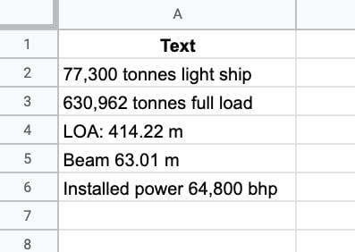
Is it possible to extract those numbers with a REGEX formula, even though they’re formatted differently?

You bet!

This formula will extract numbers with or without thousand separators and/or decimal places:

The REGEX pattern

means match any digits, commas, or periods and extract them.

So the REGEXEXTRACT formula matches the first digit it finds then keeps going with the match provided the next character is either another digit or a comma or a period, When it reaches something else, like a space or a letter, the match breaks, and the extract is completed.

We’re not quite done yet though.

Using The VALUE Function To Convert The Output To Numbers

The output of the REGEXEXTRACT formula is a string, not a number.

So we need to convert the output to a number by wrapping the result with the VALUE function like this:

The formula above is not foolproof, however.

Improving The Pattern Match

If the text string has a period or comma before the first digit then this will be extracted as the match.

For example, if the input text string was: “The ship is huge. It’s 630,962 tonnes full load.” then the REGEXEXTRACT formula from above will extract the first period only.

It matches the period after “huge” and then stops the match because of the space character that follows.

How do we modify the formula to ensure the extract begins with a number?

Well, we change the REGEX to match a number first, before anything else, like this:

Here the REGEX matches on a digit first, before looking for more digits, commas, or periods.

If you’re eagle-eyed you’ll notice that the plus + has changed to a star * after the square bracket. This means zero or more of the characters in the square brackets, to account for a situation where there is a single-digit number that we want to match.

The REGEX pattern

matches a digit, followed by zero or more characters that are digits, commas, or periods.

Now the result of the formula extraction is 630,962, which is the correct answer.

Remember, the output of the REGEXEXTRACT formula is a string, so you’ll need to wrap it with the VALUE function to convert it to a number, e.g.

Example 5: Check Telephone Numbers With REGEXMATCH

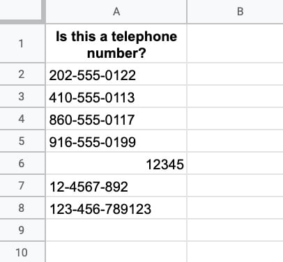
For this example, I’m going to consider US phone numbers with dashes between the sections, i.e. numbers of this format: XXX-XXX-XXXX

It’s 3 digits, then a dash, 3 digits, dash, then 4 digits.

By the end of this tutorial, you’ll have enough information to modify the example to other regions of the world.

Here’s the data:

Let’s build a REGEX formula to check whether the string in column A is a valid US phone number.

Using what we learned above, we know that the expression

matches digits. So our first attempt is this formula:

Step 1:

This matches 3 digits, then a dash, 3 digits, dash, then 4 digits and it works ok. It shows TRUE when it matches a telephone number and FALSE otherwise.

But it’s verbose. We can simplify it by using a quantifier clause.

Step 2:

The {3} means match exactly 3 of the preceding pattern, i.e. match exactly 3 digits.

This works great, except it still matches the final number on row 8. It matches the 3-3-4 and doesn’t care about the extra digits that come at the end.

But we know this isn’t a valid phone number, so how do we get it to stop after the 4 digits and discount anything with more than 4 digits in the final set?

Word Boundaries

We wrap the expression with a special expression called a word boundary, denoted by

before and after the main expression.

Technically, this matches a “zero-width nothing”. What that means is that it marks a boundary between a word character (e.g. letter or digit or _) and a non-word character. So it will match the digits up to 4 and then look for a boundary. A fifth digit will break the match, but a space won’t because it defines a boundary.

Our new expression looks like this, with a \b at the beginning and end.

Step 3:

The final thing we might do is to wrap this with an IFERROR function to handle number inputs like row 6 above that cause an error output (since the REGEX formulas only work with text strings).

Step 4:

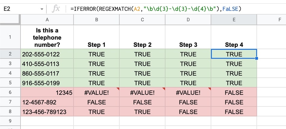
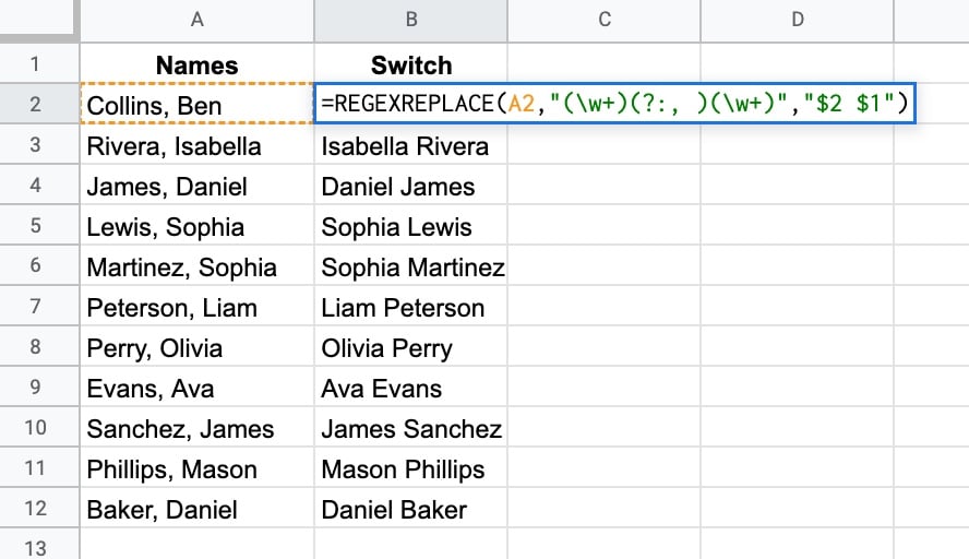
Example 6: Reorder Name Strings With REGEXREPLACE

In this example, we’re looking at the REGEXREPLACE function and a key concept in regular expressions: capturing groups.

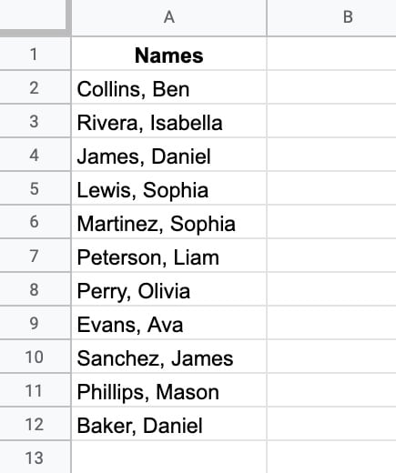
Suppose we have a list of names in this format: “Surname, First Name” and we want to switch the order to “First Name Surname”.

Here’s the formula to switch the order of the names:

Let’s break this down:

REGEXREPLACE finds all substrings that match the pattern and replaces them with the value given. It takes 3 arguments: 1) the input text, 2) the pattern to match, and 3) the replacement value.

Let’s look at each in turn:

Input text

Surname, First name e.g. Collins, Ben

Matching pattern

matches word characters.

creates a numbered capturing group. It matches the first word up to the comma.

opens a non-capturing group, which essentially means match but don’t capture the text in this group.

is the non-capturing group that matches a comma and space but doesn’t capture them.

creates a second numbered capturing group. It matches the second word after the comma and space.

Replacement Value

Now, this is where it gets interesting!

Our matching pattern captured each of the names as a numbered group, which we’re now able to refer to with

or

The group

captured the surname and group

captured the first name.

To reverse the names, we put group

first, then

The output looks like this:

SOLUTION From Example 1

Modify the REGEXMATCH formula to be:

It uses a quantifier

and word boundaries

to only match 4-digit numbers (see example 5 for more information on quantifiers and word boundaries).

Learn More

The Google Sheets REGEX Formula Cookbook

There are hundreds of more REGEX examples in my Google Sheets REGEX Formula Cookbook course.

Resources

For the full list of allowed syntax, check the re2 syntax page.