Welcome to issue 5 of the Sheets Insiders membership program.
You can see the full archives here.
This week, we’re looking at Dropdowns in detail.
We looked at these as part of the UX template in Sheets Insiders 3, but today we’re exploring them more deeply.
Enjoy!
§ Dropdowns Template
Download the Dropdowns Template
Click on “Use Template” in the top right corner to make your own copy.

The template covers four techniques:
- Automated Dropdowns
- Multi-select Dropdowns
- Dependent Dropdowns with Formulas
- Dependent Dropdowns with Apps Script
(New to dropdowns? Start here to learn the basics.)
§1 Automated Dropdowns
This is a neat trick that speeds up your dropdown workflows.
Suppose we have a long list of spending transactions that we want to categorize for analysis.
How much am I spending on eating out? How much does my car really cost me?
We could try to create all our categories in advance and set up a dropdown with the options. But inevitably, we’ll want to add to the dropdown, and this can be a pain. We have to edit it and then update all the other dropdowns too.
One way around this is to use the Dropdown (from a range) option.
And then, sneakily, we build that range with a formula that gets all the unique values from our dropdown column.
Confused? I am.
Let’s see some pictures and all will become clear.
Setup the dropdowns like this, based on the empty range in D2:D
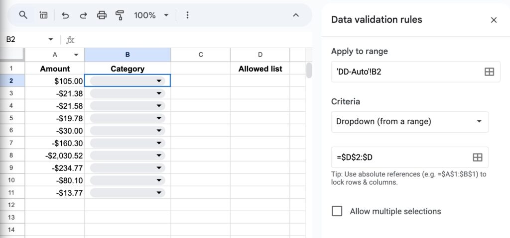
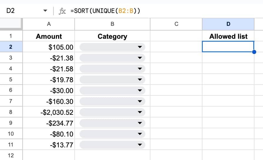
And then in cell D2, use this formula to build the list of options for the dropdown:
=SORT(UNIQUE(B2:B))
which looks like this in our Sheet:
(Adjust the ranges in the dropdown and formula if you’re using different rows and/or columns. For example, in the template, I’ve added headers so the range references have changed.)
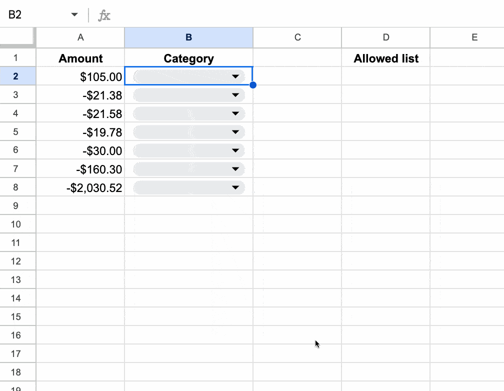
Initially, both the dropdown and the “allowed list” are empty, because they’re based off of each other.
This is where we need to jump in and start categorizing our data.
We have to add the first value.
In the first dropdown cell, type in the first category e.g. “Groceries”.
It shows up immediately in all the dropdowns!
That’s the power of this method. On any dropdown cell, we can either choose from the available dropdowns or simply type a new category and it gets automatically added to the global list.
Here you can see how it works in practice:
Thanks to Eric L. for originally sharing this tip with me.
§2 Multi-select Dropdowns
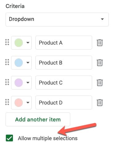
Click on the multiple selections toggle to allow users to select more than one option at a time from the dropdown:
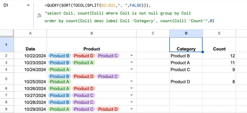
Suppose we have data set up like this:

How do we count the number of products?
Assume our data is in the range A1:B21.
Start with this formula in cell D5, to the right of the table:
=SPLIT(B2:B21,", ",FALSE)
This splits the multi-select dropdown cells.
Next, we stack the results into a single column with a TOCOL function:
=TOCOL(SPLIT(B2:B21,", ",FALSE))
We can wrap this with a SORT function, which has the nice property of giving an array output:
=SORT(TOCOL(SPLIT(B2:B21,", ",FALSE)))
Finally, we can wrap this with a QUERY function to summarize the results:
=QUERY(SORT(TOCOL(SPLIT(B2:B21,", ",FALSE))), "select Col1, count(Col1) group by Col1",0)
We can tidy the output up using some extra query syntax (optional):
=QUERY(SORT(TOCOL(SPLIT(B2:B21,", ",FALSE))), "select Col1, count(Col1) where Col1 is not null group by Col1 order by count(Col1) desc label Col1 'Category', count(Col1) 'Count'",0)
In our Sheet:
§3 Dependent Dropdowns with Formulas
Dependent dropdowns are dropdown menus where the options change based on what you’ve chosen in another dropdown.
The first dropdown in the chain is just a regular dropdown.
Subsequent dropdowns are based on ranges of filtered values, where any previous dropdowns control the filtering.
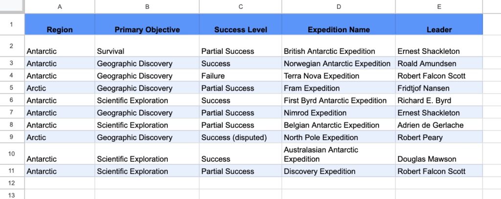
Let’s consider this dataset in A1:E11, of expeditions from the golden age of polar exploration:
And here’s the dependent dropdown in action:
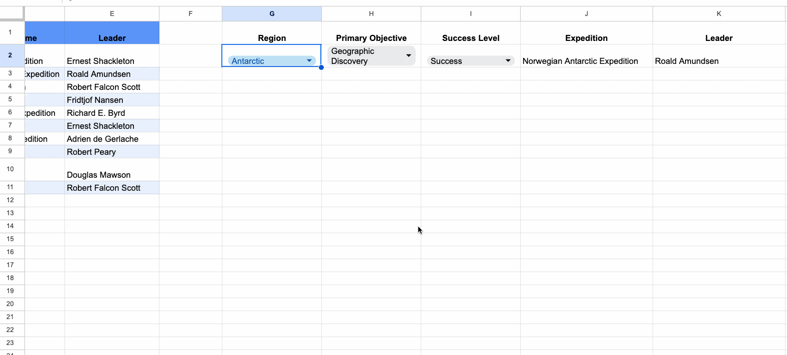
The dropdown options update when you change the choices in previous dropdowns.
They work as follows:
The first dropdown is not dependent. It’s based on the data in the first column.
Set each subsequent dropdown to “Dropdown (from a range)” and then point it to a range that contains a FILTER formula.
The formula for the second dropdown is:
=SORT(UNIQUE(FILTER(B2:B11,A2:A11=G2)))
where B2:B11 is the range of values for the second dropdown. And G2 is the choice from the first dropdown.
The next dropdown includes an extra filter condition for the previous choice (in blue), where H2 is a previous dropdown choice.
=SORT(UNIQUE(FILTER(C2:C11,B2:B11=H2,A2:A11=G2)))
Any extra dropdowns require extra filter conditions.
It’s much easier to see in the template or in this video:

Note: when you change a dropdown choice, the choices downstream of it do NOT automatically update. So it’s possible that it shows a choice that is no longer an option, and isn’t available in the dropdown menu.
Unfortunately, this is something we can’t change when using formulas alone.
§4 Dependent Dropdowns with scripts
Instead of filter formulas, we can use Apps Script to build dependent dropdown menus.
This has the advantage of avoiding the error messages when you change a filter and the previous option is not in the new dropdown.
The trick is to use the onEdit trigger to clear out the existing dropdowns and rebuild them with the new filtered choices.
Rather than explain the code line-by-line in this email, this Loom video walks through what it looks like in the Sheet, how to modify the ranges to fit your scenario, and points out some of the key steps in the code:
