1. Shortcuts
Let’s start with keyboard shortcuts. It’s one of the single best investments of time you can make to further your spreadsheet skills. It’s all about reducing your reliance on the mouse and instead harnessing the awesome efficiency of navigating spreadsheets from the keyboard.
Try these for starters:
- Quickly move around your data ranges by holding the Ctrl key (or Cmd key on a Mac) and the Left or Right or Up or Down Arrow keys. Hold down Ctrl (or Cmd) key and the Shift key with your left hand and the Left or Right or Up or Down Arrow keys.
- Move quickly between your worksheets by holding down the Ctrl key and Page Up or Page Down.
- Toggle between absolute and relative cell references using F4.
- Quickly jump into a cell to edit the contents, by pressing the F2 key.
- Highlight a whole row by holding down the Shift key and hitting Spacebar. Similarly, highlight a whole column by holding down the Ctrl key and hitting Spacebar.
Find more in the official Microsoft Excel documents for Windows or Mac.
2. Format Painter
Chances are you’ll want to re-apply format options again and again in your worksheets, for example when you’re preparing reports that need to look consistent. There’s a slow way and a quick way to do this. The slow way is to just repeat your steps each time, selecting fonts, sizes, shading, borders etc. to match.
The quick, much better, way is to use the Format painter tool and it’s really easy to use. Simply highlight the range of cells whose format you want to replicate elsewhere, then click on the paintbrush Format button in the Home ribbon tab. Then click on the cells where you wish to apply the formatting:
Pro-tip: if you double-click the painter tool when you select it, it’ll continue to be available so you can re-use again until you cancel it.
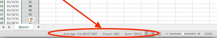
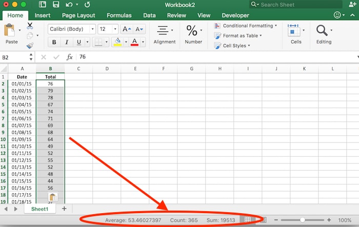
3. Use the Status bar functions
You can set up the status bar, along the base of your workbook, to display key metrics about the range of data you highlight. If you quickly want to check the sum, min, max, average of a range of data then it’s a really handy trick.
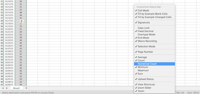
Set your status bar up by right clicking it and adding the metrics you’re interested in, like so:
4. Efficiently create column headings
Start by highlighting the whole range where you want to insert column headings. Type the first column heading in the first cell and hit Enter. The cursor will jump sideways to the adjacent cell, not down, where you can enter your next column heading.
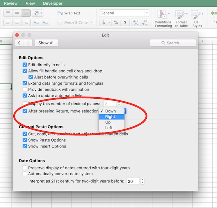
If you find yourself doing this a lot, then you can always change the setting so that hitting Enter moves the cursor to the right, rather than down. Do this by going to the Excel menu:
Preferences > Edit > After pressing Return, move selection: > Right
5. Tricks when using formulas
Use the tab key to auto-select formulas and save yourself the trouble of typing them out in full.
When you start typing a formula, you’ll see a list of possible options displayed by Excel. Use the Up and Down arrow keys to select the formula you’re after and hit the Tab key to select:
Here’s a quick way to evaluate your formulas that’s helpful for debugging when they’re giving unexpected answers:
- Select cell with your formula.
- Hit F2.
- Highlight the specific part of the formula using Shift + Left arrow, or in the formula bar.
- Press F9 to display the result of the formula.
- Press Esc keep formula or Enter to keep the value.
6. Use custom lists
Excel has built-in generic data lists (e.g. Jan, Feb, Mar, Apr,…) that you can access by dragging down one of the values (e.g. Jan) to auto-complete with the list.
Try typing “Jan” into cell A1, grabbing the handle on the bottom right of the cell and dragging down. You’ll get “Feb”, “Mar”, “Apr” etc. in cells A2, A3, A4, etc.
Well, you can also add your own custom lists. So, say for example you want to refer to the same 5 cities repeatedly in your worksheet, then add a custom list to save yourself some time.
- Go to Excel > Preferences > Custom Lists.
- Type in your new entries in the left pane.
- Click “Add” to add the new, custom list.
- Back in your worksheet, type an entry from your list (e.g. London), then drag down with the corner handle to fill the cells with your new custom list values.
7. Used named ranges
Do you ever find yourself referring to the same range of cells again and again? For example, you keep referring back to the same table in a lookup formula. Well you can name that range and then refer to it by this name, which saves you having to find and highlight the range every time.
To create a named range:
- Highlight your range.
- In the name box in the formula tab, shown in red in the image below, type in the name for your range:
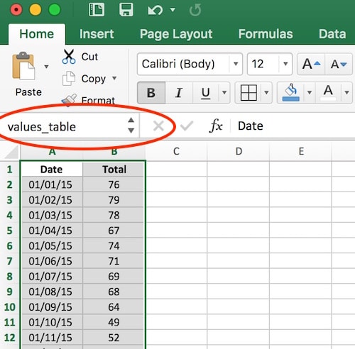
Now, when you want to refer to this table, you can simply type its name rather than having to highlight all those cell references again, e.g. in the example above I called the table values_table and I would refer to it thus:
=VLOOKUP(E11,values_table,2,FALSE)8. Use the GoTo feature to find all blank cells
The GoTo feature is a super handy way of finding things in big ranges of data, for example finding blank cells that are missing data, which you need to fill in.
- Highlight your range.
- Go to menu: Edit > Find > Go To…
- Click Special.
- Then select Blanks.
Now you have them all highlighted, you can work with this whole non-contiguous range at once, for example by highlighting them all yellow to identify them and then inserting values.
9. Use Excel Tables
Excel Tables are a powerful feature that can speed up data entry, formatting, calculating and well, just about anything else you need to do with a table of data. They’re basically a way of telling Excel that a range of data is all related and to treat it as such.
Working with Excel Tables is really slick. For example when you add a new row or column of data, Excel will auto-format it for you. Excel Tables come with Sort and Filter options already built in. If you add a calculation then Excel will fill down the whole column for you.
To setup an Excel Table:
- Highlight the range of data you want to turn into a table.
- Go to Insert > Table menu.
- Select the My Table Has Headers option if required.
- Excel will add a Table tab to your ribbon, where you can access features and formatting options.
- You can refer to ranges within your table by name now, which again speeds up your workflow, e.g.:
=average(Table1[Age])
10. Record custom macros for repeated operations
Macros are small, custom programs in Excel that you can use to create bespoke features and record common processes so that they might be easily replicated.
This is a more advanced Excel topic, so let’s just explore one example in action. As the following images show, I have a plain table of data that I format and add a new calculated column to. However, since I recorded all these steps as a macro, I can now repeat these steps with one simple mouse click.
To achieve this, you’ll need to first add the Developer Tab to your ribbon (go to Excel Preferences. Click Popular, and then select the Show Developer tab in the Ribbon check box.
Then start recording:
MS spreadsheet is most widely used, but the vast potential it has, is not fully tapped. Thanks for sharing and refreshing the knowledge.
I’m using SUMIFS where the sum_range is a named range. The problem is tha the named range varies dependant in some conditions. Apparantly, I can say ‘=SUMIFS(F15,B1:B10, “>20”, C1:C10, “<30").
Is there any work around?