Understanding Average In Google Sheets With The World’s Richest Person

This is a story about a bar, 10 regular folks, and the world’s richest man, to explore different measures of average in Google Sheets.

Somewhere along the way, we’ll seek to demonstrate the robustness of the different average measures, but more on that in a minute.

I want you to picture your favourite bar or pub.

For me, it might be a pint of ale at The Dickens Inn, near the River Thames in London:

I should just finish this blog post here, and we could all spend the rest of the day in happy reverie, supping our favourite tipple.

Alas, that won’t do! We have work to do and things to learn, so let’s get started.

The dataset

Imagine ten friends, all regular folks, sitting at the bar, eating and drinking, chatting and laughing. A most convivial scene. The beer tastes delicious of course, the floor is dappled with sunlight and the comforting aroma of Pie & Mash wafts by their nostrils. Anyway, I digress.

Let us play a little game. Our subjects don’t mind because they’re fictional.

We ask them all to write down their salaries in our Google Sheet, so we have the following results:

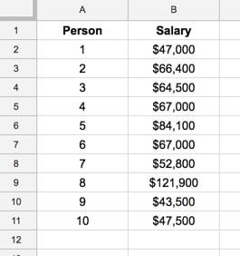
Good. That’s our dataset.

Calculating the average in Google Sheets

You can use formulas or pivot tables to calculate averages. In this post, I’ll show the method using formulas, since it makes it easier to focus on what’s happening with the average measures.

We then calculate the “average” salary, using the three different measures we know:

Mean Average in Google Sheets

Using the formula

we calculate the mean — the classic average — of our data. This calculation is the total of all the values divided by the count of how many there are.

The mean of this dataset is $66,170

It’s the measure of “middle-ness” or “central-ness” that we’re perhaps most familiar with.

However, there are two other common average measures:

Median Average in Google Sheets

Using the formula

we calculate the median, or middle value, of our data.

If we have an odd number of values, this value is just the middle value that bisects our data into two evenly numbered groups.

If we have an even number of values, as we do in this example with 10 people, then the median is the mean of the middle two values.

In our case, the middle two values, when the data is sorted, are $64,500 and $66,400. We add these two together, which is $130,900, and divide them by two to give us the median value.

The median of this dataset is $65,450

Mode Average in Google Sheets

Using the formula

we calculate the mode — the most frequent value — in our our data.

The mode of this dataset is $67,000

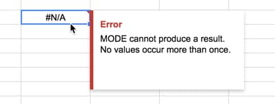
Note: if none of the values in your dataset occur more than once, then no mode can be calculated and the Google Sheets function will produce an error:

So far so good.

This is where we introduce the world’s richest man.

His name is Jeff Bezos and he’s worth approximately $120bn, that’s right 120 BILLION DOLLARS. It’s hard to fathom how much money that is, but suffice to say that quitting his lucrative Wall Street job to found Amazon 23 years ago has paid off handsomely.

For the sake of this exercise, we’re going to assume Jeff has an annual salary of $10 million dollars (the majority of his $120bn wealth is his ownership stake in Amazon).

Now, suppose Jeff has just finished some stressful meetings in London and decides to avail himself of a pint of beer. He just happens to choose the same pub as our 10 friends from earlier.

After the awkward ensuing silence and subsequent predictable astonished whispers (“He looks like… Is that…? Wait, is it really…?”), normal service resumes and Jeff pulls up a stool at the end of the bar.

He is subject number 11 in our dataset, which, if we include Jeff’s salary, now looks like this:

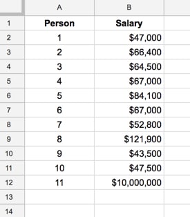
Whew, that’s an outlier if ever I saw one.

And it has a HUGE impact on one of our averages, but which one?

The effect of outliers on mean, median and mode

Taking our new dataset of 11 values above, let’s calculate the mean, median and mode again.

The new mean is $969,245

The new median is $66,400

The new mode is $67,000

Wow! Look at that mean value now.

It’s jumped from $66,170 to $969,245. Now, if we were to say the average salary of all the folks in this room was almost 1 million dollars, you’d jump to all sorts of wrong conclusions.

The mean has been skewed so dramatically by the outlier, that it’s become a rather meaningless number now. It’s highly sensitive to outliers.

However, look at the median, which has barely changed, and the mode, which hasn’t changed at all. The median and the mode are what we call robust statistics. They have not been skewed, or unduly affected, by the new outlier.

Average Conclusion

We’ve seen how the mean is sensitive to outliers, and this is its principal drawback. It’s not a robust statistic. As we saw in our example, it was skewed so much that the result was essentially meaningless.

The advantage of the mean is that it can be calculated on discrete (example above) and continuous data (e.g. people’s heights).

The median, being the middle value that bisects the dataset, is less affected by outliers, so is a better measure of central tendency when the data has outliers or is not symmetrical.

The mode, being the most frequent value, has the principal advantage that it can be calculated for numerical and categorical (non-numerical) data.

It’s also possible to have no mode (no values occur more than once, which can happen with continuous data), two modes (bimodal distribution), or even many modes (multi-modal).