Sheets Insiders 35: Reader Ideas! -

Welcome to issue 35 of the Sheets Insiders membership.

This week, we’re looking at suggestions you submitted, in response to last week’s email. Thanks to all readers who submitted tips! 🙏

And, WOW! 🤩

We’ve got some zingers, so enjoy!

They’re listed in ascending order of difficulty, with the easiest tips at the top. My personal favorite is the clever dynamic SUM formula at the bottom of the list, so be sure to read to the end.

1. Shortcut F4 to lock references

Quickly toggle between relative and absolute references in formulas with the F4 key.

Press the F4 key when your cursor is touching a range reference:

Thanks Heidi for this one!

2. Version History

Go to the menu File > Version history > See version history

Use it to restore older versions if something goes wrong.

You can also name versions to track milestones.

Thanks, Paul!

3. Highlight Incomplete Rows

This tip highlights any rows that are incomplete or missing data:

Highlight your data and go to the menu Format > Conditional Formatting

Enter this custom formula rule:

=COUNTBLANK($B2:$D2)<>0

Change the range to match the first row of your range. Note the “$” before each column letter, which are required to make it work.

Thanks, John!

4. Comments with Global Conditional Formatting

Sticking with Conditional Formatting for a moment…

Highlight your entire Sheet (by clicking that little box at the top left, between the “A” and the “1”.

Then go to the menu Format > Conditional Formatting

Add this custom formula rule:

=LEFT(A1,2)="//"

Change the format to highlight the cell background orange (or whatever color you like!).

Now, anytime you type “//” at the beginning of a cell, it will highlight it in a special way!

These cells now stand out as sort of de facto global commenting protocol in your Sheets.

Thanks, Ernesto!

5. Use LET for complex formulas

LET is an incredibly useful formula, allowing you to create variables that can be reused. It’s invaluable when creating complex formulas because it lets you store the results of intermediate calculations for reuse.

Here’s an example where we store the value of an AVERAGE function in a named variable “av” that can be reused:

=LET( av , AVERAGE(B2:D2) , IFS( av>80 , "Distinction" , av>60 , "Good" , av>40 , "Pass" , TRUE , "Fail" ))

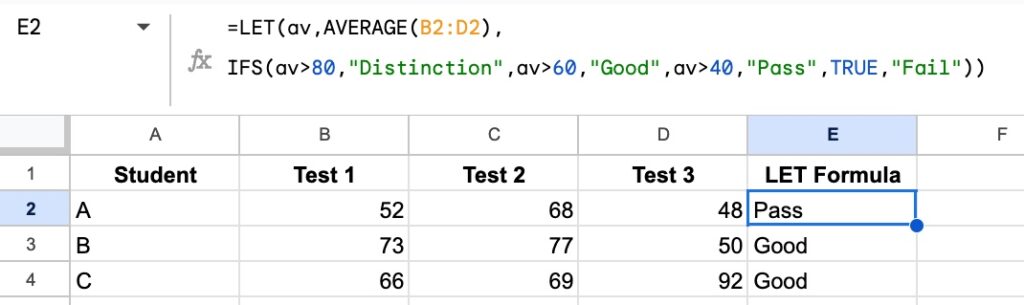
Learn more about the LET function.

Thanks Steve for suggesting the LET function!

6. Filter with Partial Match

To illustrate this example, I’m using a table called “content” that contains a list of webpages.

This FILTER + REGEXMATCH formula will extract any pages with the word “Google Sheets” in the Title column:

=FILTER( content , REGEXMATCH( content[Title] , "Google Sheets" ))

It looks like this in our Sheet:

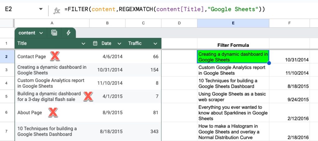
The red Xs indicate rows that are excluded by the filter because they don’t contain the words “Google Sheets”.

Thanks, Kim!

7. Dot Chart

Here’s a nice, easy way to add a visual touch to your data.

Use the IF and REPT functions with red and green emojis to create a simple dot chart:

=IF(A2=0, "🔴", REPT("🟢", A2))

In our Sheet:

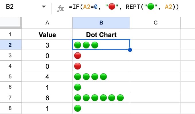
Thanks, Paul!

8. Dynamic Sum with the INDIRECT Function

This special SUM formula automatically includes new values.

Compare the dynamic SUM formula on the left versus a regular SUM function on the right:

The formula is:

=SUM(A2:INDIRECT("A"&ROW()-1))

If the SUM formula is moved down, the dynamic version will automatically include any new data that is added.

The regular SUM function does not. The range reference will need to be updated.

To be sure, this adds complexity to a regular formula, so I’m not advocating you make all your SUM formulas dynamic.

But for niche scenarios, it might be useful. Or perhaps it gives you ideas of how else you can use the mysterious INDIRECT function.

Thanks Edward for this clever formula!

Template

Download the Reader Suggestions Template >>

Click on “Use Template” in the top right corner to make your own copy.

There is no Apps Script with this template.