This tutorial will show you how to combine text and numbers in Google Sheets, and keep the the correct number formatting in place.
Combining text and numbers is common in spreadsheets, for example when you want to add some context, e.g.:
Total: $5,250
Discount: 35.5%
However, if you try to combine text with numbers (or currencies/percentages/dates) directly in a cell in Google Sheets, you’ll notice the numbers loses any formatting, which will make the number harder to read or even less meaningful, e.g.:
Total: 5250
Discount: 0.355
You can use the TEXT function to fix this, and apply formatting to numbers that are displayed with text in a cell.
Combine Text And Numbers In Google Sheets
To combine text, in a cell or denoted by quotes "Text", and numbers, use the TEXT function, as shown in these examples.
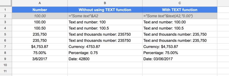
For these examples, I’m assuming I have numbers, currency numbers, percentages or dates in column A:

What’s the formula?
With numbers in column A, then you can combine text and numbers with:
="Text and number: "&text(A1,"0.00")="Text and number: "&text(A2,"#.##")What’s the difference?
The 0 forces your cell to display zeros if a number has fewer digits than the format specifies, whereas the # does not force the display of zeros.
So TEXT(19.9,"000.00") displays 019.90, whereas TEXT(19.9,"###.##") displays 19.9.
For a deeper look at number formatting in Google Sheets, read my Google Sheets custom number format tutorial.
Thousands separator
If your number is in the thousands, and you want to show the thousand separator comma, simply add that into the format section of the text formula. It works the same for the “0” or “#” notation:
="Text and thousands number: "&text(A3,"0,000")="Text and thousands number: "&text(A3,"#,###")Currency
Combining text and currency is easy enough, now you know how to format numbers. Simply add the currency symbol to the front of the number and it will show in your text:
="Currency: "&text(A4,"$0,000.00")Percentages
Combining text and percentages:
="Percentage: "&text(A5,"0.00%")Dates
Combining text and dates:
="Date: "&text(A6,"mm/dd/yyyy")
Hello
What if A has any value text or number and I want to add comment “finish” on B
Ben, my dates all turn out like this: 12/30/1899
Here is my formula:
=ArrayFormula(if(Z2:Z””,”StudentId: “&Z$2:Z
&char(10)&”Role: “&AD$2:AD
&char(10)&”Address: “& AE$2:AE
&char(10)&”Entering Year: “& AJ$2:AJ
&char(10)&”Entering Grade: “& AK$2:AK
&char(10)&”Checklist Item: “& AM$2:AM
&char(10)&”Date Requested: “&text(AN$2:AN,”mm/dd/yyyy”)
&char(10)&”Date Due: “&text(AO$2:AO,”mm/dd/yyyy”)
&char(10)&”Date Completed: “&text(AP$2:AP,”mm/dd/yyyy”)
&char(10)&”Date Waived: “&text(AQ$2:AQ,”mm/dd/yyyy”)
&char(10)&”School Program: “&AR$2:AR
&char(10)&”Checklist Name: “&AS$2:AS
&char(10)&”Par 1st Nm: “&AT$2:AT
&char(10)&”Par Lst Nm: “&AU$2:AU
&char(10)&”Par Email: “&AV$2:AV))
Can you see my mistake?
Many thanks (loving your courses, by the way).
Brian
I need this for mixed where second column needs to reference number only such as :
A | B |
1 Amp| =A:A*2 |
Returns:
1 Amp|#ERROR
Your solution applied: 1 =TEXT(“Amp”)
Returns:
#ERROR|#ERROR
(Error: Formula Parse Error)
I’m confused. What do I need to do?
Oh, I see. My example needed to be changed. It still does not resolve the second column.
1&”Amp” Returns:
1 Amp | #ERROR (Error: Function MULTIPLY parameter expects numbers. But “1 Amp” is a text and cannot be coerced to a number)
Can you have a currency and a percentage representation in the same cell?
For example: 46%, $460
You bet Shane, to separate the two use this as an example:
If you want it to take the math you’ve already done.
=text(B1,”$#.##”)&”, “&text(B2,”0.00%”)
Or you could even get the calculations returned by replacing b1 or b2 in the example with the sum(a1*a2)
Hi, I’m trying to put text in front of a squence but the methods I have tried seems to block the squence function. I have tried this:
="WEEK "&SEQUENCE(10,1,1,1)But it just outputs: ‘WEEK 1’ in one cell rather than all 10 rows.
Can you help Please.
Hi Shivaraj,
Turn it into an array formula and it’ll output all 10 rows for you:
=ArrayFormula("WEEK "&SEQUENCE(10,1,1,1))Cheers,
Ben
Thank you Ben!
I’ve figured out how to use this except for inputting time into text. Is there a way to correctly format time in hours and minutes (00:00)?
Every time I reference a time with text, it turns it into a decimal value of 24 hours. Example; 6:00 = 0.25. 12:00 = 0.5. and 24:00 = 1. Even when combining this with the text function (=text(B2,”0:00″), it does not display the correct time, but instead a tiny fraction of the correct time.
Any help is greatly appreciated!
Hello again.
I just figured out my question using the formula below. I could not have done that without your website. Thank you so much!
=text(B2,”H:MM”)