Welcome to issue 31 of the Sheets Insiders membership.
You can see the full archives here.
This week, we’re looking at arrays in Google Sheets. An array is a collection of elements in rows and/or columns.
Using arrays is a great skill to master because they’re useful for presenting data and generating complex formulas. And, once you get the hang of the syntax, they’re really not hard to use.
Introduction
In the programming world, an array is a data structure that stores elements sequentially in memory. You can think of it as a list.
In Google Sheets, the definition is a little more vague, but essentially an array is a collection of data. It can consist of data in rows or columns or both.
Where arrays really come in handy is when you use them to combine formula outputs.
We’ll get to that. But first, let’s cover the basics of array construction.
How to create arrays in Sheets
We can construct arrays with curly brackets, { }, which we call array literals, or with the modern HSTACK and VSTACK functions.
Today, we’re going to focus on the { } construction. They’re more succinct than the functions, but either works.
To construct basic arrays, use curly brackets with commas (European countries use backslash instead) and semicolons.
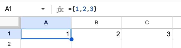
Commas create a row array:
= { 1 , 2 , 3 }
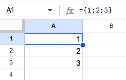
whereas semicolons create a column array:
= { 1 ; 2 ; 3 }
These can be combined. E.g. using a mixture of numeric and string values in this example:
= { "X" , 100 ; "Y" , 200 ; "Z" , 300 }
which looks like this in our Sheet:
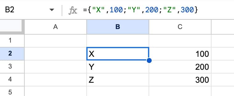
So, commas “,” create horizontal arrays (across columns). And semicolons “;” create vertical arrays (across rows). And mixing them together creates 2-D arrays.
The number of elements in each row and/or column must match. I.e. if the first row has 3 elements, then every other row must also have 3 elements.
(* Note: in European countries, the syntax is different. Use a backslash “quot; instead of a comma “,” to separate the horizontal arrays. More info here.)
Now, let’s look at some practical examples:
Example 1: Column Headings
I see this often as a way to “hide” formulas in column headings.
This makes them less likely to be accidentally deleted or unintentionally broken versus if they were mixed in with the data.
The syntax is:
= { "Column Name" ; data }
This stacks the words “Column Name” on top of the data.
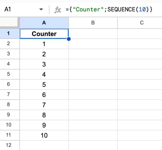
For example, this formula in A1 creates a column with 10 numbers:
= { "Counter" ; SEQUENCE(10) }
Example 2: Add a total row to a QUERY function
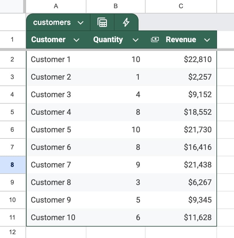
Consider this Table, which is called customers:
We might write a QUERY function like this:
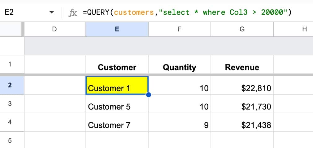
=QUERY(customers,"select * where Col3 > 20000")
which gives this output:
Suppose we want to add a total column. How?
Well, we would write a SUM function like this:
=SUM(QUERY(customers,"select Col3 where Col3 > 20000"))
Now, the first formula outputs a table with 3 columns. But the second formula only outputs a single number. So, we can’t combine them in an array yet.
We need to turn the second formula into an array with 3 columns, which we can do like this:
={ "Column 1", "Column 2", SUM(QUERY(customers,"select Col3 where Col3 > 20000")) }
Let’s rename “Column 1” as “Total” and “Column 2” as a blank value “”.
The formula becomes:
={ "Total", "", SUM(QUERY(customers,"select Col3 where Col3 > 20000")) }
which looks like this in our Sheet:

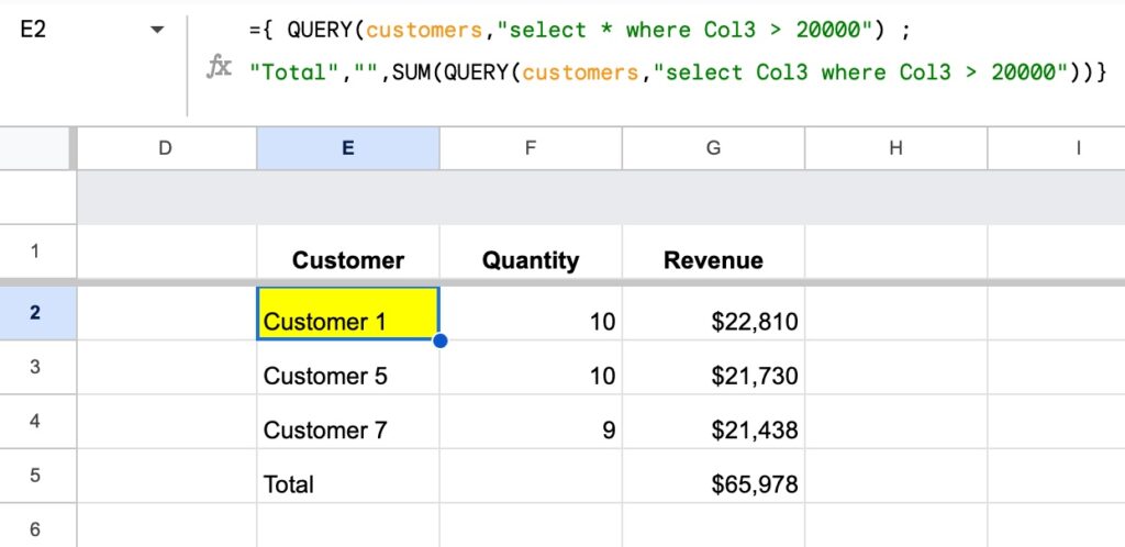
Now we can now combine these two formulas with the array { } like this:
={ QUERY(customers,"select * where Col3 > 20000") ; "Total" , "" , SUM(QUERY(customers,"select Col3 where Col3 > 20000" ) ) }
BONUS: this formula can be improved with a LET function, like so:
=LET( data,QUERY(customers,"select * where Col3 > 15000"), { data ; "Total" , "" , SUM(CHOOSECOLS(data,3) ) } )
The LET makes the formula shorter by letting us put the QUERY output into a variable called “data” that can be used in multiple places in the array.
Example 3: Sparkline with word overlay
In Monday’s newsletter, I promised a formula that would bring some *dazzle* to your Sheets.
Here it is:
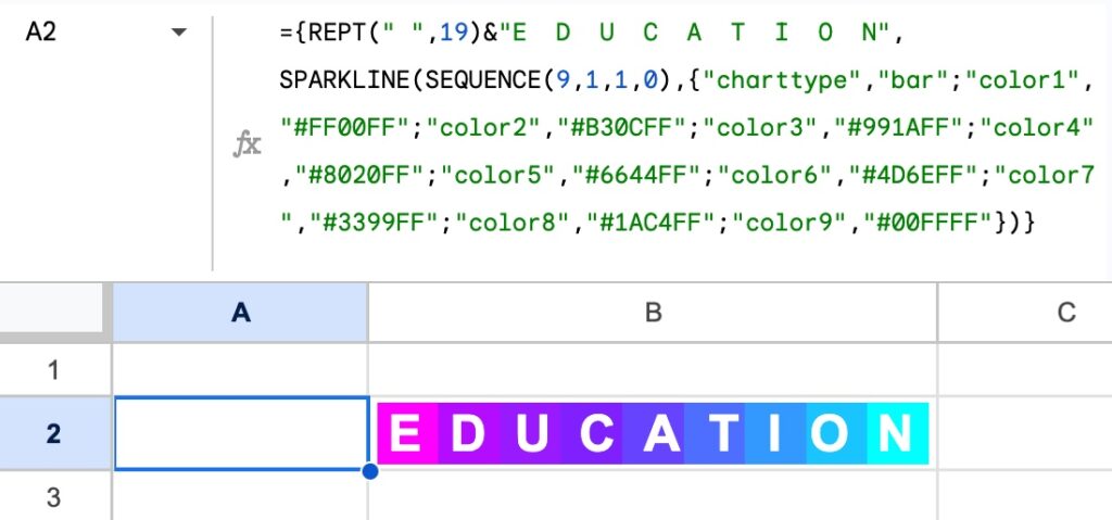
And here’s the single formula in cell A2 that creates the entire image and word in B2:
={ REPT(" ",19) & "E D U C A T I O N", SPARKLINE(SEQUENCE(9,1,1,0) , { "charttype","bar" ; "color1","#FF00FF" ; "color2","#B30CFF" ; "color3","#991AFF" ; "color4","#8020FF" ; "color5","#6644FF" ; "color6","#4D6EFF" ; "color7","#3399FF" ; "color8","#1AC4FF" ; "color9","#00FFFF" } ) }
How it works:
- The outer { , } creates a row array with two elements.
- The REPT() function creates a buffer of spaces that pushes the word to the right until it overlays the sparkline.
- The SPARKLINE formula consists of two parts: 1) an inner SEQUENCE function to generate a list of nine 1’s for the data, and 2) an array of color combinations.
There is a longer explanation of how this works in the video above.
Some notes on usage:
- The sparkline and text appears in the cell next to the formula. I.e. if you enter the formula above into cell A1, the sparkline appears in B1.
- Keeping this in mind, you format the text by changing the formatting on the formula cell. For example, change A1 to white and size 15 and it will affect how the text shows on top of the sparkline.
- Feel free to change the word “E D U C A T I O N” to whatever word or words you want to show.
- Change the value inside the REPT function (currently 19) to adjust how far across the word is pushed.
- Feel free to remove colors from the array inside the sparkline. Currently, it goes up to “color9”, which is the maximum number.
- Feel free to change the hex values inside the sparkline to use different colors.
Template
Download the Arrays in Formulas in Google Sheets Template
Click on “Use Template” in the top right corner to make your own copy.
There is no Apps Script with this template.