I was going through my emails yesterday and saw one about Google’s new Pixel 10 phones. Curious, I clicked the link and browsed the site for a while.
It’s a nice, clean site with dropdown menus and columns of data.
Hmm, I thought, could it be recreated in a Google Sheet?
Trying to recreate something in Google Sheets is a great way to learn new skills and get design inspiration.
It forces you to think outside the box to achieve a certain look or action.
(This is the same message I shared in my regular newsletter last year #315: Design inspired by lightning!)
Pixel phone website recreated in Sheets
Take a look at the new Pixel 10 website so you have the original source of inspiration.
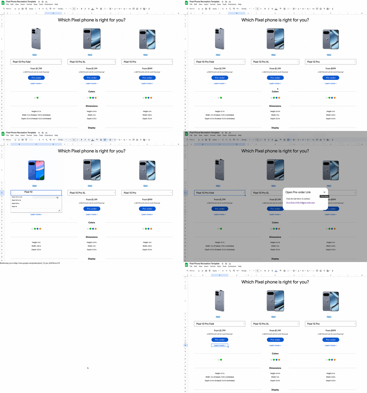
And here it is, recreated in a Google Sheet:

We’re going to look at a bunch of different techniques that all come together to create this template.
Let’s start with the design elements and then talk about the data elements.
1. Design Elements
The original website has the phone data organized into 3 columns, so I knew that I could match that. I used additional columns to create the space between the three columns.
More whitespace created breathing room around sections to give the sheet a clean, professional look.
I used the Google Sans font to match the Google look. Subtle borders around the dropdowns and between sections helped define headers and separate areas without adding clutter.
I used dropdowns to add interactive elements that allow users to select the phone model. Then the IMAGE function lets me add the phone image into a cell, based on the selection in the dropdown.
=IMAGE( XLOOKUP( B9 , urls[Phone] , urls[Image URL] ) , 4 , 295 , 370 )
I used a Table called “urls” to store the URLs of the images, then I use the XLOOKUP to retrieve the URL based on the phone selected in the dropdown. The number “4” in the IMAGE function lets me set a custom size.
Hiding the gridlines instantly makes any reporting sheet look more polished and app-like, so it made sense for this scenario.
Finally, I added a footer with a link back to my website, so people know who made the Sheet and can get in touch if they need to.
(Since this is an SI template, I also added the customary Info Sheet to the front. Here’s the Sheets Insiders tutorial from January on how to automate this.)
2. Data Elements
The first step was to use the IMPORTHTML to scrape the data from the Pixel website. Here’s the formula:
=IMPORTHTML("https://store.google.com/magazine/compare_pixel?toggler0=Pixel+10+Pro+Fold&toggler1=Pixel+10+Pro+XL&toggler2=Pixel+10+Pro&hl=en-US","table",1)
Once I had the live data in my Sheet, I made a hardcopy version. Copy the data to a new sheet using Paste special > Values only. I recommend doing this because when (not if) the data changes on the source website, your IMPORT formulas will break.
Then I created a formula that takes two inputs:
- the phone choice (from the dropdown)
- the section header (e.g. dimensions, or display, or camera, etc.)
and returns the relevant specs for that phone and that category.
Here it is:
=LET(
phoneChoice, TRIM(A1),
idx,XMATCH(phoneChoice,CHOOSEROWS(phoneSpecs,1)),
phoneChosen,CHOOSECOLS(phoneSpecs,idx),
infoRequest,XLOOKUP(A2,CHOOSECOLS(categories,1),CHOOSECOLS(categories,2)),
TRANSPOSE(SPLIT(CHOOSEROWS(phoneChosen,infoRequest),CHAR(10))))
This formula takes a phone name (in A1 for example) and a category (in A2 for example), then pulls the matching details from my data.
First, it uses TRIM to trim the phone name, finds which column matches that phone in the header row with XMATCH, and isolates that whole column of specs with CHOOSECOLS.
Next, it uses XLOOKUP to find the chosen category in the categories table to find the row where that category’s specs live.
With the phone’s column and the category’s row references, the formula extracts the relevant cell with CHOOSEROWS.
It splits the text by line breaks into separate pieces with SPLIT, and transposes them vertically into a clean list with TRANSPOSE.
Finally, it uses LET for structure.
Urgh, it’s an absolute BEAST of a formula.
Thankfully, I converted this into a Named Function to save my sanity.
Find Named Functions under the menu: Data > Named functions
I called the new Named Function “Pixel”:
=PIXEL(A1,A2)
Compare using this new function versus the behemoth above!
The last piece of functionality I wanted to build was to include buttons that opened up the relevant pre-order pages, just like on the real site.
To do this, I inserted Drawings (menu Insert > Drawing) that looked like buttons.
Then, I added a script to each button (here’s how to do that).
The script architecture looks like this, with one script for each button and one main processing function that takes the phone name and creates the pre-order link popup.

Due to security restrictions, Google Apps Script can’t directly open a new browser tab.
Instead, the script displays a small pop-up dialog box containing a clickable link to the webpage.
See the template below for the full code.
Template
Download the Pixel Phone Recreation Template >>
Click on “Use Template” in the top right corner to make your own copy.
There is Apps Script with this template.