This post is an exploration of what’s possible with formulas alone.
I’m going to use formulas to create a dynamic table of contents that updates automatically when you change the sheet names.

The key to it all is the CELL function, which can extract the address of a cell.
Extracting Sheet Names Automatically
I start with a Google Sheet containing two sheets.
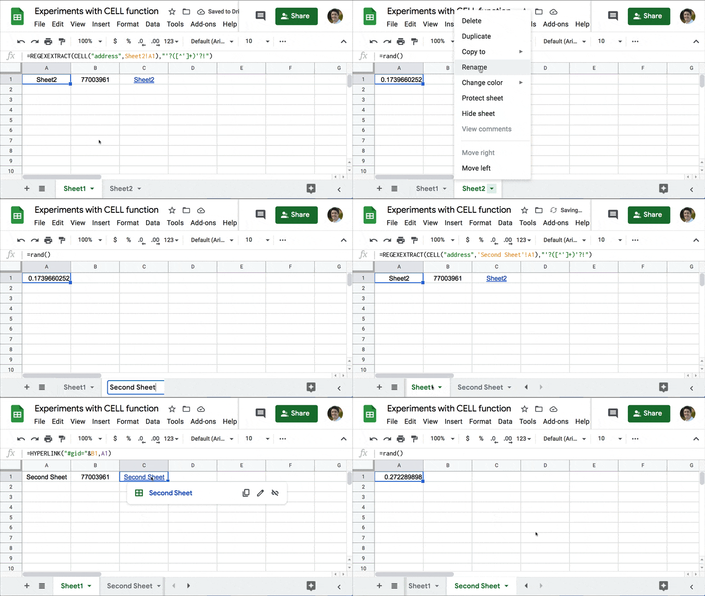
On Sheet2, I put the RAND function in cell A1:
=RAND()Back in Sheet1, I put this formula into cell A1:
=CELL("address",Sheet2!A1)It gives me this output: Sheet2!$A$1
Using a simple Google Sheets REGEX formula, I can extract just the Sheet name:
=REGEXEXTRACT(CELL("address",Sheet2!A1),"'?([^']+)'?!")This changes the output to just show the Sheet name: Sheet2
Now pay close attention, here’s the next key step. I switch the spreadsheet calculation to every minute.
File > Spreadsheet settings > Calculation > On change and every minute
Now, when I change the name of Sheet2 to something else (e.g. “Dataset”), the cell value in Sheet1 will change within the minute.
If you’re a nerd like me then that’s super cool.
It’s happening automatically, without me intervening.
I’ve used a formula to extract information that is outside the rows and columns of my actual Sheet.
Internal Google Sheet Links With The Hyperlink Formula
Normally you use the HYPERLINK function to link to external sites or for “mailto” links, basically external links.
To do internal linking within a Google Sheet, you click on the cell and create a special link.
It looks and feels like a hyperlink but it’s not formula driven, so can’t be used in conjunction with the CELL function technique above. Moreover, the text in the link doesn’t change.
However, there is a way to create internal links with the hyperlink function.
Each sheet (tab) within your Google Sheet has a unique #gid appended to the URL, shown here in red:
https://docs.google.com/spreadsheets/d/XXXXXXXXXXXXXXXXXXXXXXXXXXXXXXXX/edit#gid=77003961Use this #gid number from the Google Sheets’ URL inside the hyperlink function.
Sheet1 (or the “first” sheet in your Google Sheet) has the number 0.
Other sheets have longer #gid numbers, e.g. 349283867
I copied this #gid number for Sheet2 into Sheet1, in cell B1, next to the CELL formula.
Then in cell C1, I constructed this hyperlink formula:
=HYPERLINK("#gid="&B1,A1)This creates a working hyperlink that takes me to Sheet2 if I click on it.
Even better, if I change the name of Sheet2 to “Second Sheet” or “Dashboard” or “Leaderboard” or whatever, the link will automatically update and I can still click through to this second sheet.

This technique reminds me of the methods to create dynamic named ranges in Google Sheets. Use a side-effect of a regular function to do something interesting.
Create A Dynamic Table Of Contents With Formulas
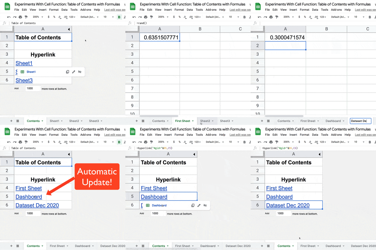
Taking this a step further, I used this technique to build a live table of contents that always displays the correct sheet names.
It updates every minute or whenever a change is made.
Admittedly, it’s a lot of work for a not enormously useful result, but it’s still an interesting and unusual application of programming with formulas.
The last change is to hide the two helper columns containing the REGEX formula and the #gid number, to make it look more like a table of contents.
Of course, it still requires a random number in a destination cell on each sheet, for the REGEX function to reference. And I have to set the calculation to “on change and every minute”, as discussed above.
(You can always hide the random number cells by formatting the text white for example.)
As always, I’d love to hear your thoughts in the comments below!
Hi Ben,
I’d just recently signed up to your free advanced formulas course, (which is excellent I might add). I mention this as I’m new to google sheets and had to post on Googles doc forum to get help with a formula with a hyperlink within a sheet. There someone also mentioned your name (in a positive way I might add), so that’s how I found you,,,, (I know you really wanted to know all that!) 🙂
I’ve just read the above, and now read that when hyperlinking within the same workbbook, I can now do this just by referencing ‘#gid’ instead of the full doc URL!
Brilliant stuff!
You are a God! 🙂
Keep up the great work Ben.
Best regards
John C
THIS IS AWESOME
Hi Ben. I have individual SOURCE files that I link to a separate overview ‘Aggregator’ file. In the SOURCE file TEMPLATE there is a hyperlink in a cell named “File”. This is IMPORTRANGE into Aggregator view as a quick way of jumping to the SOURCE file. Is there a quick way of puling the spreadsheet URL in to each new SOURCE file created from the TEMPLATE, or does it need to be done manually each time.
I started working with Excel in ca. 1995, simple macros, etc… I switched to Google Sheets 4 years ago, so I’m quite an avid spreadsheet user for 25 years, uninterrupted.
Ben, your site is the very best in this topic – IMHO by far. Very useful examples, cristal clear, but not too lenghty explanations. Congrats and a big thank you!
Thank you, David! Appreciate your kind words and support.
So admittingly, my initial read was very cursory and I had skimmed due to time constraints. The very first formula ended up tripping me up, and I had to double-back and re-read. Just to confirm if I’m interpreting this accurately, is the purpose of the `rand()` function purely as a means to autonomously trigger a continuous poll as to update to the sheet from server-side with no local/user/other actions/dependencies?
Yes! That’s it. Since the Sheet is set to recalculate every minute, I need something that will automatically update and force a refresh of the CELL function.
Cheers,
Ben
BEN this is solving a huge problem for me as its now 2023 and my appscript uses webhooks to check for updates to forums.
thats about all the code I need really to builda dynamic site and app as many over complicate app build with zapier and money money money automations. But what you are doing here well solves my inablity to hide the simplicity .
Now without giving away specifics I will explain how you helped.
And will help others I know for sure to keep their blogs updated and worthy of researching lol. A top 10 or 20 or 100 is a form of table of contents and the TOPs will never change so being able to reference the TOP lets say 10 trending colors of summer 2023, this is great a the table of contents will not change but the colors will by sales data, therefore every summer by end of may the list can autogenerate and your 2024 will change as the old 2023 data was backed up automatically and now your blog just webhooked the change to update one of your more popular articles in which you only had to write one time as if done write you can refill the contents that can automatically update how to use certain colors in a scheme that is also data driven cause color schemes are pretty common and dont variate from the rules of cordination. I personally care less about paint. But the thing im going to use it for very much so relies on a weekly automated update and was dreading having to share the sheet with clever ways to using sheets without paying for a database as I like to reserve that for the backups such as the 2023 summer colors to save on money when it comes to that monthly app payment. cutting the fat with a sheet is what im all about. SO again sorry for the lengthy explanation but I see things of how they can be useful and this struck a chord on my cello. Maybe others will now understand how very much so important this is and can be used to simplify their articles and create a dynamically written blog if done write amongst ten thousand other uses I can see this for. THANK YOU BRO…wind beneath my wings and all.
PS instead of rand for A1 I adjusted for top 100
which is simple enough to be Clear column and format to number then RANDARRAY(1000,1) scooch over a few decimals to 10000ths to be safe and randomize my “ROW A” which is now “ROW AA” cause it was driving me crazy and indeed ALL WHITE LETTERS I have a header so named the header ID in “RED” and Hide. Row 1 headers,
My Top 20 Column A Row 2, + Your Formula (never changes)
Column B Row 2″ my weekly date” webhooked dynamic data
with Column A my #1-#20 row(3-23), +Your Formula (*static)
my Column B rows (3-23)
Forgot to explain the magic for me is dispursing this over and over as the data for each web app for each show using the app which is 100s is different therefore having to change the tab names is mandatory, now with this formula I can create my template with all 30 tabs of data for each show and know that no two apps will share the same tab name as each needs to be unique to the database its being utilized thru. Would have left me requiring code in a database now I just need to implement a command to rename all tabs
Thanks for sharing