The VLOOKUP function is a super popular formula but suffers from a major drawback. You can’t lookup data to the left!
However, there’s a sneaky trick that lets us VLOOKUP to the left, so we can search for a term and return a result from a column to the left of the original search column:
How do we create a VLOOKUP to the left?
What we do is create a new virtual table with an array, where the columns are switched, so the VLOOKUP can work on this temporary, virtual table.
What’s the formula?
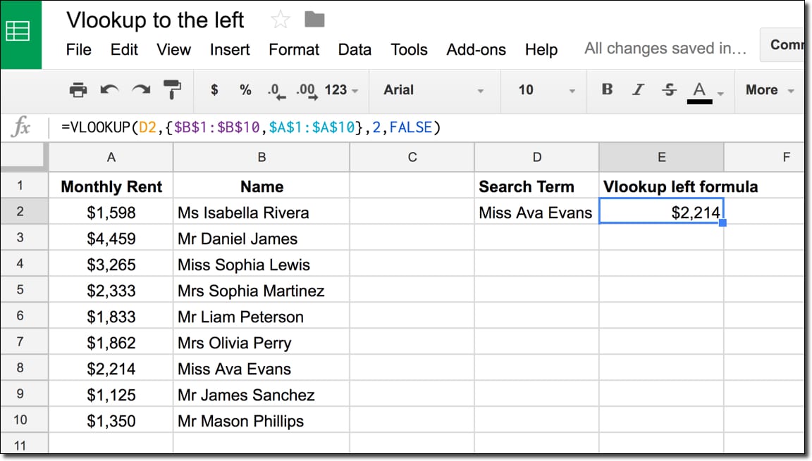
Let’s assume we have data in columns A and B. I want to search column B and return the value from column A, then we use:
Can I see an example worksheet?
How does the VLOOKUP to the left formula work?
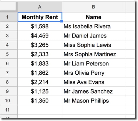
Imagine this is your raw data table and you want to search for a name and return the rent figure:
The first step is to use an array literal formula to create a new table on the fly, and then perform the VLOOKUP on this new temporary table.
This formula creates the temporary table:
as shown in the following image:
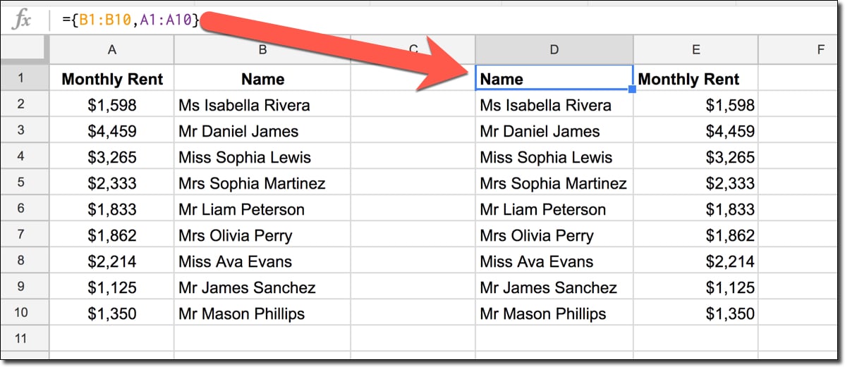
This formula has curly brackets to denote an array and inside, the two columns are swapped. This creates an array output with the two columns reversed.
Note, they don’t have to be adjacent columns, they just happen to be in this simple example.
Next, this formula performs a vlookup on the new temporary table (which is all done inside the vlookup, so you won’t actually see the temporary table):
which effectively performs a search like so:
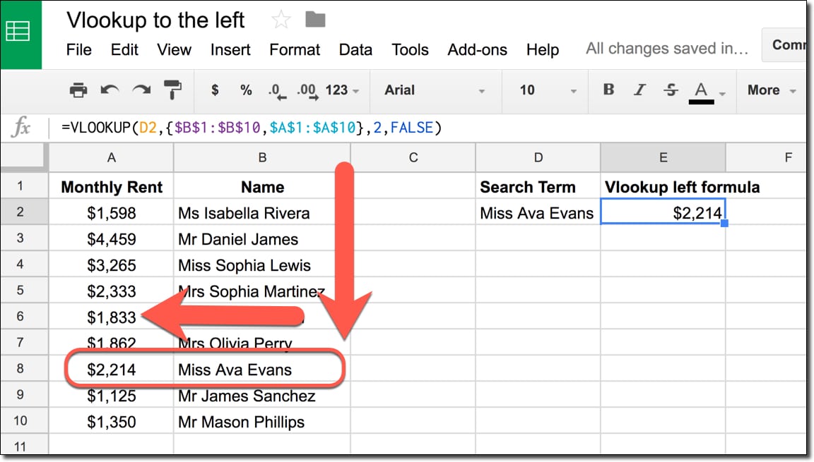
Bingo!
It returns $2,214 as we want.
Note: A better way to solve this is by using a combination of the INDEX and MATCH functions. See Day 10 of my free Advanced Formulas 30-day Challenge course.
See also how to have VLOOKUP return multiple columns.
All-matches, un-ordered lookup:
=FILTER(A:A, B:B = $E$2)
First-match, un-ordered lookup:
=INDEX(A:A, MATCH($E$2, B:B, 0))
First-match, ordered lookup: (fastest by n^2 rows)
=INDEX(A:A, MATCH($E$2, B:B, 1))
Will it work if the range A1:A10 Contains drop down list? If not why?
# Thanks in advance
Great tip and so simple!
THANK YOU SO MUCH
Hi, the formula ={B8:B17,A8:A17} doesn’t work in my Google Sheets. Instead of returning a table of 2 columns, mine returns a table with 1 column: column B and below column A. Any idea about how to solve the issue?
Hi Caterina,
Are you based in Europe? If you are, your syntax is ={B8:B17\A8:A17}
Otherwise, I’m not sure what’s happening. You could try using the XLOOKUP function, which is better for left lookups anyway: https://www.benlcollins.com/spreadsheets/xlookup-function/
Hope this helps!
Ben