SUBTOTAL Function in Google Sheets

The SUBTOTAL function in Google Sheets is a powerful function for working with data.

There are three principal uses for the SUBTOTAL function:

1. Calculating Subtotals for lists of data
2. Calculating metrics with filtered and/or hidden rows of data
3. As a dynamic function selector

It’s versatile, as you’ll see in this tutorial.

However, it’s not well known and I suspect it’s vastly under utilized. It’s not an easy function for beginners to use, because it involves using a function code to control how it operates, as you’ll see below.

SUBTOTAL function template

Click here to open view-only copy >>

Feel free to make a copy: File > Make a copy…

If you can’t access the template, it might be because of your organization’s Google Workspace settings. If you click the link and open in an Incognito window you’ll be able to see it.

Now, let’s consider the syntax:

SUBTOTAL Function Syntax

It takes two or more arguments: first the function code, then at least one range of data to operate on.

The function code is a number that determines what operation the SUBTOTAL function will perform on your data. For example, the number 9 corresponds to the SUM function.

An example SUBTOTAL formula might be:

Notice the number 9 as the first argument of this function, meaning this particular example will apply a SUM function to the range A1:A10.

There are 11 different function behaviors accessible with the SUBTOTAL and for each, you specify whether to include or ignore any hidden rows of data.

If the function code number is between 1 – 11 the hidden rows are included in the calculation.

If the function code number is between 100 – 111 the hidden rows are ignored in the calculation.

Note: rows of data that are filtered out are never included in a SUBTOTAL, regardless of the function code.

Here are all the options available for the function code option:

Aggregation	Code, including hidden values	Code, ignoring hidden values
Average	1	101
Count	2	102
Counta	3	103
Max	4	104
Min	5	105
Product	6	106
Standard Deviation	7	107
Standard Deviation Population	8	108
Sum	9	109
Variance	10	110
Variance Population	11	111

Using The SUBTOTAL Function To Create Subtotals

Suppose you have the following dataset, where each sub-table has a subtotal using the SUM function:

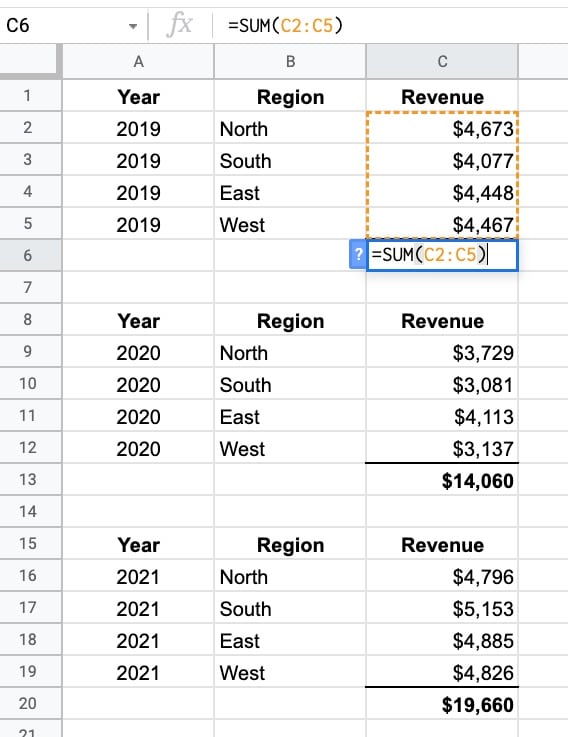
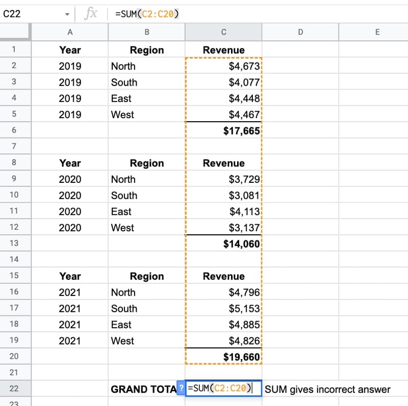
If you calculate the grand total using the SUM function, you risk double counting the revenue.

The SUM function adds the revenue values AND the subtotals, meaning your total will be twice what it should be. This is BAD!

To fix this, you have to manually select the subtotal values and sum them with a formula like this:

This isn’t ideal because it’s tedious to select each one and easy to make a mistake.

However, by using the SUBTOTAL Function in Google Sheets, you can solve this problem.

Replace each of the SUM formulas with formulas using the SUBTOTAL function, e.g.:

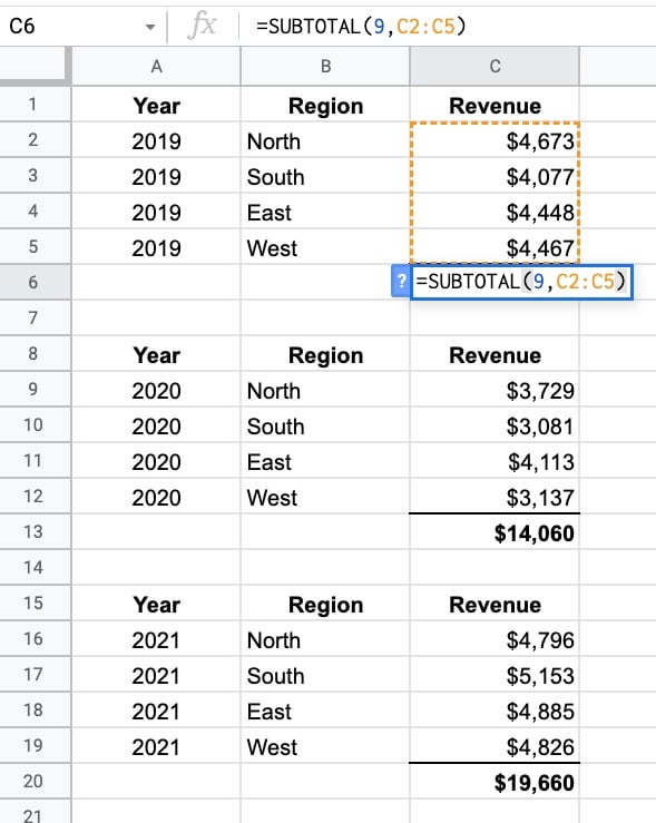
When you calculate the grand total, again using the SUBTOTAL function, it won’t double count the values. The SUBTOTAL function ignores the other SUBTOTAL functions in the table above:

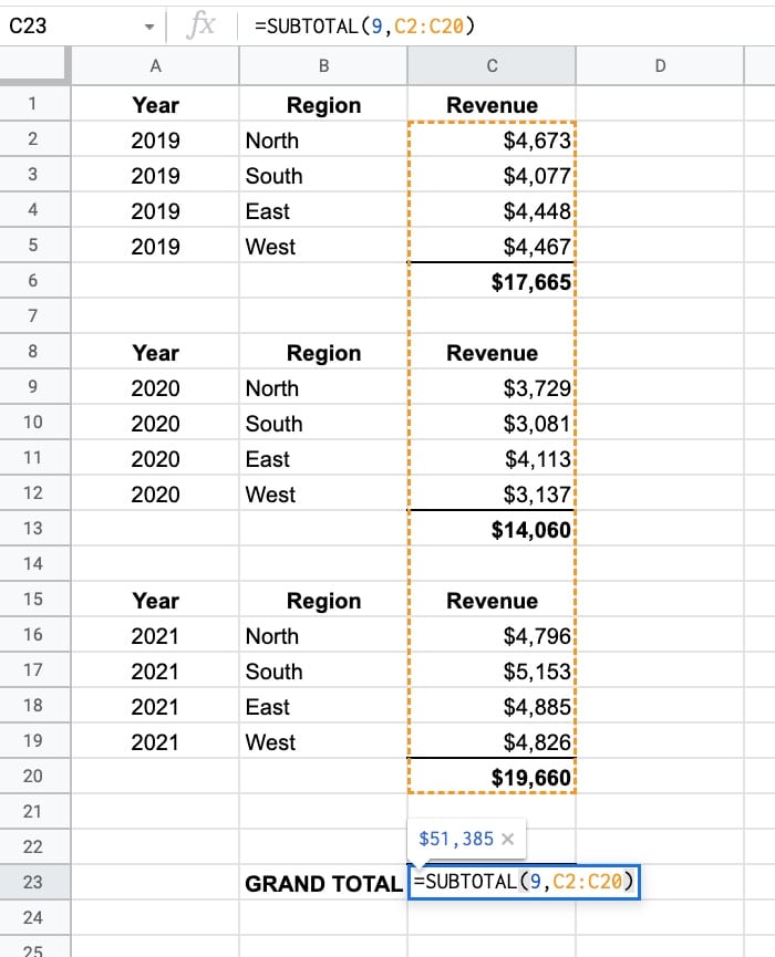
This time it gives the correct answer of $51,385

Note: Generally, it’s a better idea to use pivot tables to analyze your data and calculate subtotals. They’re much more flexible and quicker to use.

Using The SUBTOTAL Function For Filtered Or Hidden Data

Suppose you have this dataset:

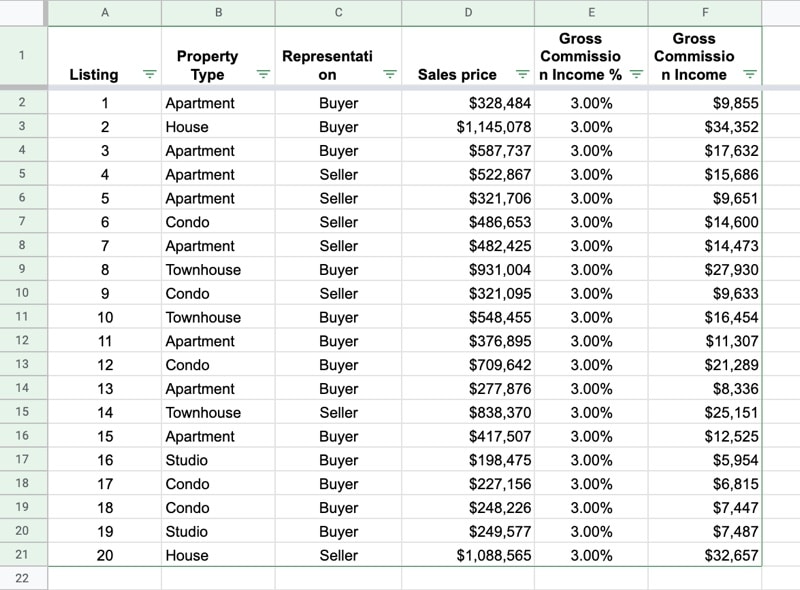
And you have these three formulas under the data:

Filtered Data

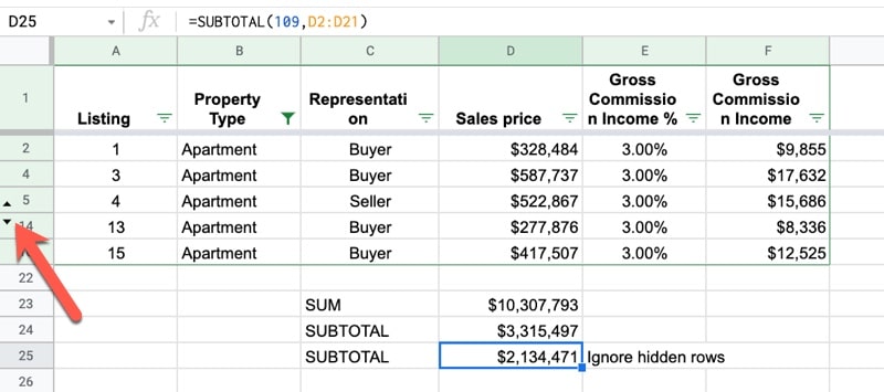
Using the filter feature, we’ve selected “Apartment” from the Property Type.

The SUM formula does not change and still returns the total of the whole dataset.

The two SUBTOTAL formulas update though and now only show the total for the filtered subset of data. They have the function codes 9 and 109 respectively, which both denote the SUM operation.

Hidden Rows

If we now hide some rows as well, by highlighting them, right-clicking and selecting “Hide rows…”, then the output of the final SUBTOTAL function updates.

Because it has the function code 109, it now ignores the hidden rows as well, whereas the formula with the function code 9 does not.

Note On Hidden Columns: The SUBTOTAL function does not account for hidden columns. If you’re using SUBTOTAL across a row then it always includes all the columns. For that reason, it’s intended for use on lists of data in column format.

Create A Dynamic Function Selector With A SUBTOTAL Formula in Google Sheets

Using the function code table above as a lookup table, you can build a dynamic selector so the user can choose which function to apply in the SUBTOTAL:

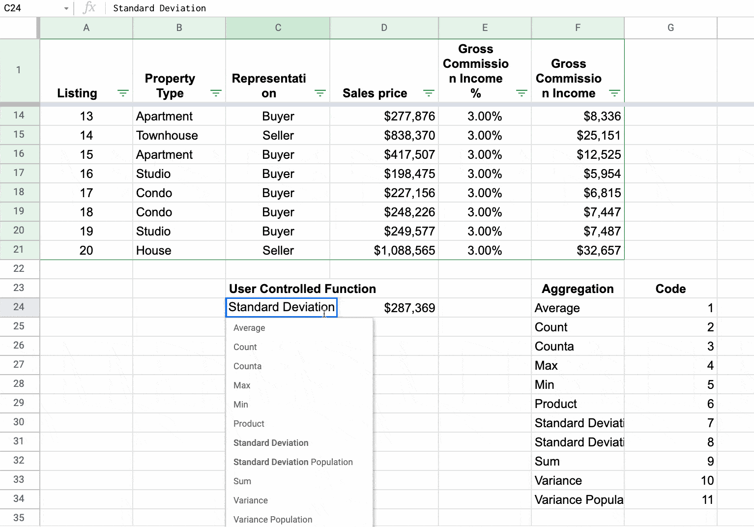
First, create a drop-down list from the list of aggregation methods in the function code table using data validation.

Select a blank cell (in this example C24) and go to the menu: Data > Data validation

Select the drop-down option and highlight the aggregation names (i.e. Average, Count, Counta…) as the range.

This VLOOKUP formula will return the code based on the drop-down item chosen:

Feel free to use an INDEX-MATCH (or even just MATCH!) instead of the VLOOKUP if you prefer. I’ve used VLOOKUP because for most people, it’s more familiar.

This code can then be plugged into a SUBTOTAL formula:

It’s also possible to add another drop-down so the user can choose whether to include or ignore hidden rows:

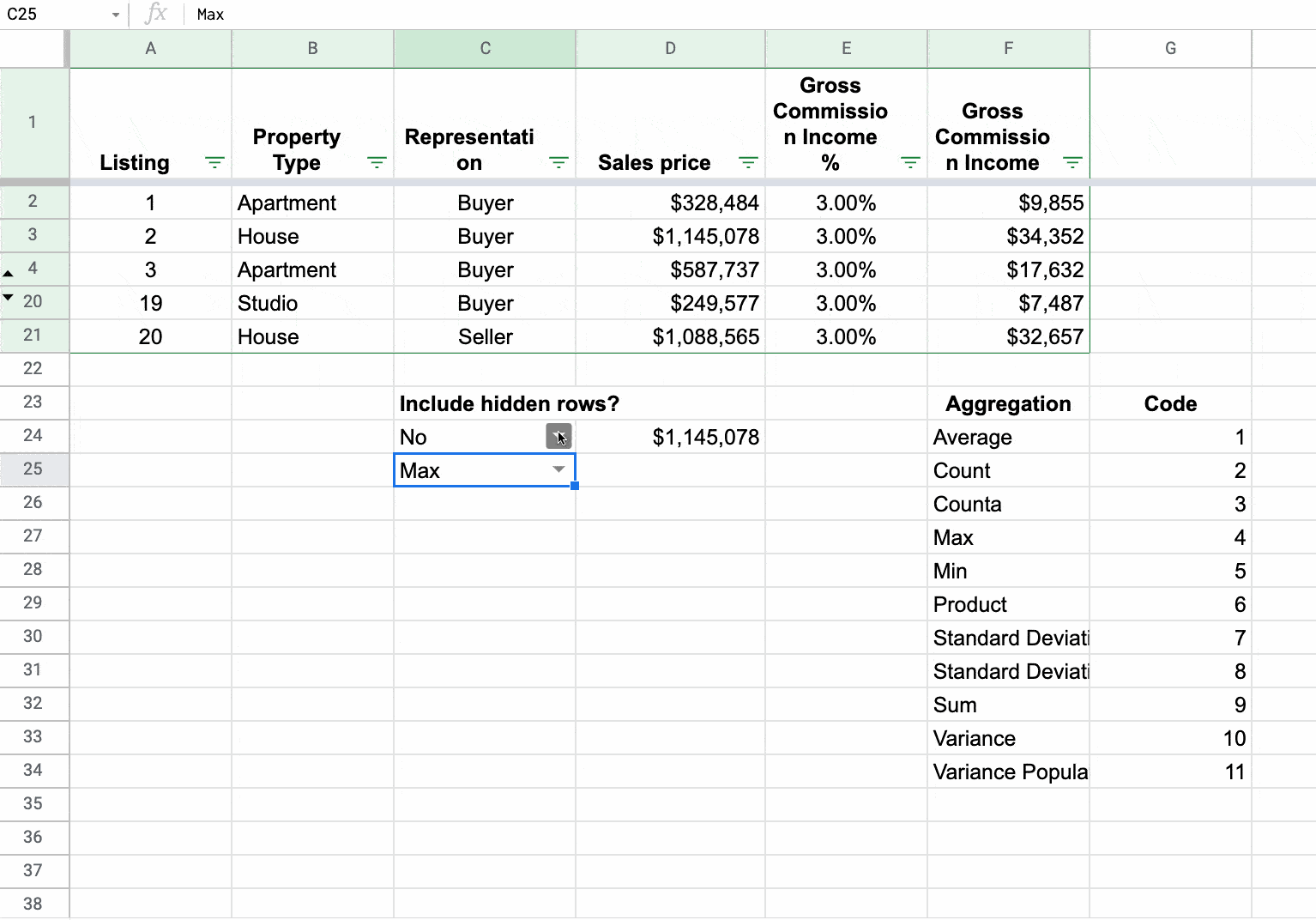
This is accomplished by including an IF function:

This gives an answer of 0 or 100, which can be added to the function code to select either the 1 – 11 range or the 100 – 111 range (see the function code table at the top of this article).

The full, dynamic SUBTOTAL formula becomes:

The SUBTOTAL function is also covered in the Day 27 lesson of my free Advanced Formulas 30 Day Challenge course.

You can also read about it in the Google documentation.