 💡 Learn more
Learn more about working with Lambda Functions, Named Functions, and X-Functions in the FREE Lambda Functions 10-Day Challenge course
The REDUCE function in Google Sheets turns an array input into a single value, by applying a custom LAMBDA function to each value of the input array.
It reduces an array down to a single value.
It’s best to understand through a simple example:
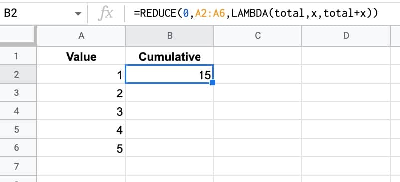
The formula in this example is:
=REDUCE(0,A2:A6,LAMBDA(total,x,total+x))The REDUCE function takes a starting value (0 in this example), an input array, and then a custom LAMBDA function.
The formula applies the custom LAMBDA function to each value in the array. In this case, it takes the current total value and adds the next value in the array to it to make a new total. This new total is passed on to the next iteration.
So this REDUCE formula calculates the cumulative total of the 5 numbers.
(And yes, this formula also gets you there:
=SUM(A2:A6)This REDUCE was deliberately simple to show you how it works.)
🔗 Get this example and others in the template at the bottom of this article.
REDUCE Function Syntax
=REDUCE(initial_value, array_or_range, lambda)The REDUCE function repeatedly applies a lambda expression to each value in the input array, moving row by row. Each intermediate value is accumulated into the accumulator. REDUCE returns the result in the final accumulator.
It takes 3 arguments:
initial_value
This is the starting value of the accumulator.
array_or_range
This is the input array or range of data to be reduced.
lambda
The custom LAMBDA function that will be applied to each value in the input range. The LAMBDA function must have 2 name arguments and 1 function expression.
The first name will evaluate to the current result in the accumulator. The second name resolves to the current value of the input array.
REDUCE Function With Array Literal Inputs
The REDUCE function accepts array literal inputs, which are arrays created with curly brackets {…}.
This is the same example as above, but uses an array literal as the input, rather than a range of data in the Sheet.
The output in this case is the value 15.
=REDUCE(0,{1,2,3,4,5},LAMBDA(x,total,total+x))Each number is passed into the LAMBDA and added to the accumulator.
REDUCE Formula Numbers Example
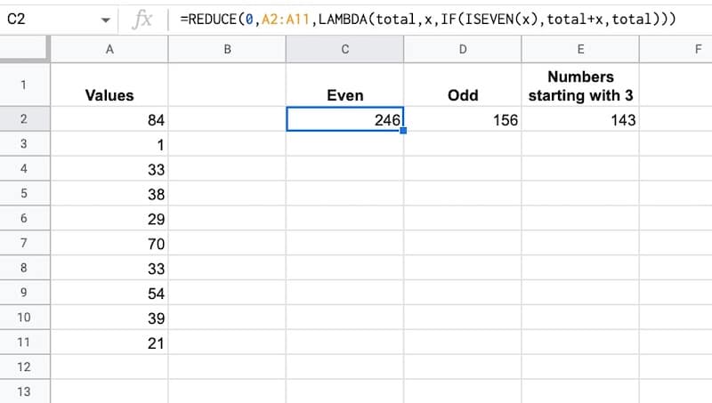
Suppose we have an array of values (e.g. 84, 1, 33, 38, 29,…) and we want to sum various different combinations.
This reduce formula will sum the even numbers:
=REDUCE(0,A2:A11,LAMBDA(total,x,IF(ISEVEN(x),total+x,total)))And this one will sum the odd numbers:
=REDUCE(0,A2:A11,LAMBDA(total,x,IF(ISODD(x),total+x,total)))What if we wanted to sum numbers that began with 3?
We could use this reduce formula to sum numbers that began with 3:
=REDUCE(0,A2:A11,LAMBDA(total,x,IF(LEFT(x,1)="3",total+x,total)))In all three cases, the accumulator starts with the value 0 and then each value in the array is evaluated by the lambda function. If the test inside the IF statement is true, the new value is added to the accumulator, but if it’s false, it’s not added.
Advanced REDUCE Formula Example
Consider this dataset of names with titles:
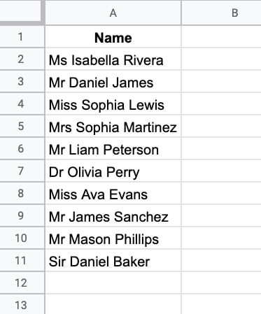
Now suppose we want to remove all of the titles?
One way is to use the SPLIT function on the spaces and then re-join the names. But let’s see how to do it with the REDUCE formula instead.
First, we need an array literal of the different titles, which will be the input array for our reduce formula.
{“Mrs”,”Mr”,”Ms”,”Miss”,”Dr”,”Sir”}
Then we set the initial value to be the first name, so the reduce looks like this:
=REDUCE(A2, {"Mrs","Mr","Ms","Miss","Dr","Sir"}, LAMBDA(...))Inside the LAMBDA, we want to use the SUBSTITUTE function to replace each array value in the initial value with a blank character.
SUBSTITUTE(value,title,"")For example, suppose we start with this value: “Ms Isabella Rivera”
Next, we take each value in the array literal of titles and, one by one, see if we can substitute it into this initial value.
The result is the name without the title, i.e. “Isabella Rivera”
The full REDUCE formula is:
=REDUCE(A2, {"Mrs","Mr","Ms","Miss","Dr","Sir"}, LAMBDA(value,title,TRIM(SUBSTITUTE(value,title,""))))The TRIM function is included to remove the leading space.
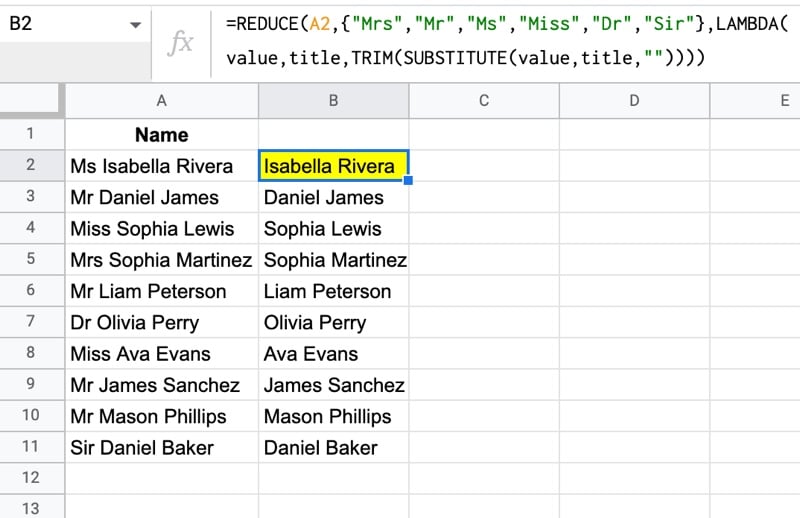
This can also operate as an array function to clean up an entire array of names with a single formula:
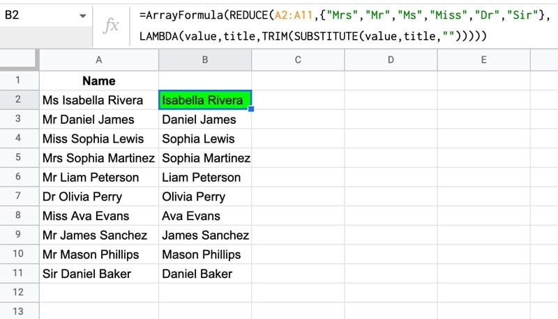
Note: the order of the elements in the array literal is important. The “Mrs” must come before the “Mr”, otherwise the reduce will substitute “Mr” into “Mrs Sophia Martinez” to leave “s Sophia Martinez”.
REDUCE Function Template
Click here to open a view-only copy >>
Feel free to make a copy: File > Make a copy…
If you can’t access the template, it might be because of your organization’s Google Workspace settings.
In this case, right-click the link to open it in an Incognito window to view it.
See Also
See the LAMBDA function and other helper functions MAP, REDUCE, MAKEARRAY, etc. here:
On my regular Google account, the maximum permitted number of calculations for Reduce is 39,998. Reduce is not available yet on my Workspace account to test if it is the same. I used this formula to test it: =reduce(0,sequence(39998),lambda(x,n,x+1/n))
A number of calculations that large noticeably slowed down the spreadsheet. When I tried just 1000 iterations, I did not notice any slowing.
I’m pretty sure that Reduce and Sequence could be used as a sort of for…next loop based on the length of the Sequence, preferably for much shorter Sequences. The Sequence number need not even affect the action performed; it can just be a counter to establish the length of the loop.
Pretty soon, we’ll be able to pack a whole spreadsheet in cell A1. 🙂
Thanks for sharing this info, Mike! Interesting find.
Is it possible to have a function return a series of REDUCE outputs in an array?
I’m trying to turn a monthly % change into an annual change. To do this I need to do (1+A2)*(1+A3)+(1+A4)… through all 12 months of the year.
I figured out how to reduce that into one query: =REDUCE(1,A2:A12,lambda(accumulator,current_value,(current_value+1)*accumulator))
Now what I’d like to be able to theoretically do, is have another arrayformula on top of that that would apply to all my dates on a rolling basis. I can easily drop the formula down, but am wondering if there’s a fancier way to do this.
I was searching for a way to consolidate datatables from multiple tabs into a single tab using a range of sheet names (which the user could maintain).
Here’s a solution using reduce() and vstack() …
=reduce({“Name”,”Gender”,”Job”},A1:A2,lambda(DataTable,SheetName,vstack(DataTable,query(indirect(SheetName&”!$a:$C”),”select * where Col1” and Col1’Name'”))))
In the lambda function, DataTable contains the result so far (starting with an array of column names), SheetName is the next sheet from the range of sheet names, indirect and query pull the next set of data, stripping off the column headers, before vstack adds the data to the DataTable.
I would never have thought about doing it this way without your examples – keep up the great work!
Nice one, Steve! Glad to hear the resources are helpful. Keep up the great work yourself too!
I have found an interesting way to apply a replacement table to a text.
To do this, the first column of a replacement table is run through line by line and all occurrences of the characters in a text are replaced with a SUBSTITUTE function. I need this to convert special characters from ISO-Latin 1 to ASCII characters.
The replacement table contains the characters to be replaced in the 1st column and the replacement characters in the 2nd column.
=REDUCE(“TEXTÁÄÆ”,INDEX(replacement-table,0,1),LAMBDA(_text,_char,SUBSTITUTE(_text,_char,ARRAYFORMULA(XLOOKUP(TRUE, EXACT(_char, INDEX(replacement-table,0,1)), INDEX(replacement-table,0,2))))))
Based on the “Mr/Mrs” example, I used the REDUCE function to replace a list of special characters.
The replacementtable is a two-column list. The first column contains the characters to be replaced and the second column contains the characters to be replaced. Name can contain special characters that are to be replaced. (Special characters (Latin 1 addition), e.g. À by A, È by E, ç by c, Ö by Oe, ö by oe, …)
=LAMBDA(_text,_table,
REDUCE(_text,INDEX(_table,0,1),
LAMBDA(_text,_char,
SUBSTITUTE(_text,_char,
ARRAYFORMULA(XLOOKUP(TRUE, EXACT(_char, INDEX(_table,0,1)), INDEX(_table,0,2)))
)
)
)
) (name;replacementtable)
I’m not entirely satisfied with the function, as you have to search for the letter to be replaced in a somewhat “laborious” way. Unfortunately, I don’t know any way of finding out which line the REDUCE function is currently in. Or is there one?
With kind regards
If sum(a2:a6) can achieve what =REDUCE(0,A2:A6,LAMBDA(total,x,total+x)) can, why not use sum(a2:a6)?
Hi Mael,
It’s just a simple example to illustrate how the function works. I think it’s helpful before jumping into the more complex real-world use cases.
Cheers,
Ben