How To Draw The Sierpiński Triangle In Google Sheets

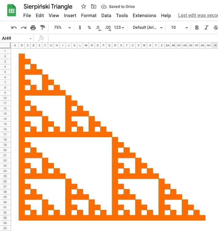
The Sierpiński triangle is a fractal set in the shape of an equilateral triangle, divided into smaller triangles infinitely.

Graphically, we can draw an approximation of the Sierpiński triangle in Google Sheets:

🔗 Get this example and others in the template at the bottom of this article.

It is named after the Polish mathematician Wacław Sierpiński and is also known as the Sierpiński gasket or Sierpiński sieve.

It has the property of being self-similar, meaning it looks the same at any magnification.

See Wikipedia for more on the Sierpiński triangle.

The Sierpiński Triangle In Google Sheets

There are many different methods to construct the Sierpiński triangle.

Perhaps the easiest method to visualize is the removing-triangles method.

Start with an equilateral triangle, subdivide it into four smaller triangles and remove the central triangle. Repeat with each smaller triangle an infinite number of times.

However, we use a different method — Pascal’s triangle — to draw an approximation in Google Sheets.

Construction In Google Sheets

Pascal’s triangle is a triangle made up of numbers where each number is the sum of the two numbers above. The Sierpiński triangle is a modified version where a modulo 2 operation is performed after the addition.

Step 1:

Firstly, add additional columns up to AH so that our drawing can be 32 cells wide by 32 cells tall.

Step 2:

Next, highlight all your columns and reduce the width so they’re squares.

Step 3:

In cell B2, add the value 1. This is the value in the top left corner of the triangle.

Step 4:

In cell C2, add this formula:

and then drag it across the row to cell AG2.

The MOD function in Google Sheets returns the result of the modulo operator, the remainder after a division operation.

Step 5:

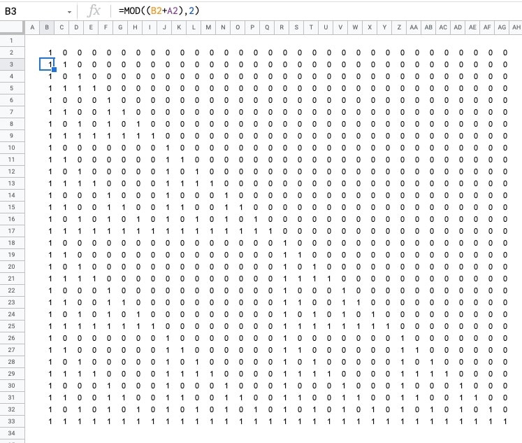
In cell B3, add this formula:

Drag down the column to cell B33.

Step 6:

Next, highlight the formulas in cells B3:B33 and drag across the rows to column AG.

Following these 6 steps, you should have a grid of 1’s and 0’s as follows:

Step 7:

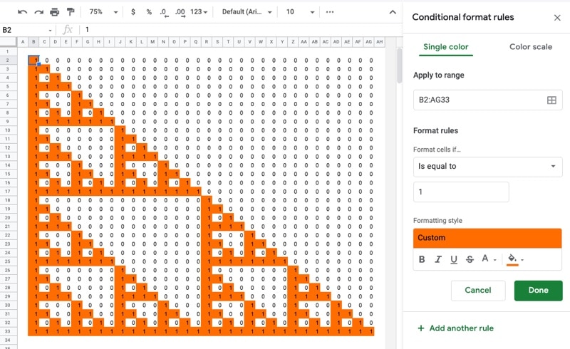
Highlight the 32 by 32 grid — the range B2:AG33 — and add conditional formatting.

Go to the menu: Format > Conditional formatting

Set the format rule to “Is equal to” and a value of 1.

Change the background color to something bold, e.g. orange.

Step 8:

As a final step, let’s remove the numbers.

We’ll use a custom number format to do this.

Go to the menu: Format > Number > Custom number format

Set the custom number format to:

;;;

This tells your Sheet to hide any values in the cells, so the 1’s and 0’s don’t show.

To finish, you can also remove the gridlines from the menu: View > Show > Gridlines

Sierpiński Triangle Variations

By changing the divisor number in the MOD formula, you can explore the fractal nature of the Sierpiński Triangle.

Follow the same steps as above, but modify the formulas so that the divisor in the MOD function is $A$1 rather than 2. For example, the formula in cell C2 is:

Then in cell A1 put the value to be used as the divisor. Start with 2 as you set the Sheet up, but then feel free to experiment with different numbers.

To see the effects, you need to update the conditional formatting rules. Either: i) set up a new rule for each number, or ii) use the color scales (easier method).

Method 1: Conditional Formatting Rules

Here I set conditional formatting rules for each value up to 12, i.e. I created a rule for 2 as we did above, then replicate it for 3 but with a different color, then 4, then 5, etc.

Look closely and you can see me change the value in A1, which changes the values of the formulas and subsequently changes the formatting applied too.

Method 2: Color Scale

And here’s a variation using color scales within conditional formatting to achieve a similar effect:

Both of these examples are available in the template below.

Sierpiński Triangle Template

Click here to open a view-only copy >>

Feel free to make a copy: File > Make a copy…

If you can’t access the template, it might be because of your organization’s Google Workspace settings. If you right-click the link and open it in an Incognito window you’ll be able to see it.

See Also

How To Draw The MandelBrot Set In Google Sheets

How To Draw The Cantor Set In Google Sheets

Exploring Population Growth And Chaos Theory With The Logistic Map, In Google Sheets