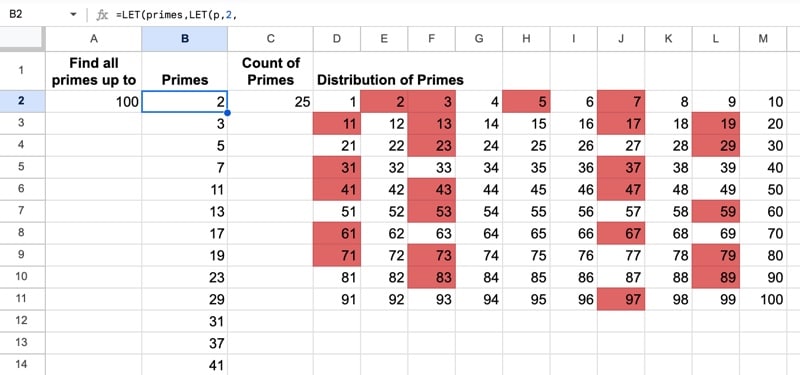
Recursion in Google Sheets is now possible with the introduction of Named functions, LAMBDA functions, and LET functions. In this post, we’ll explore the concept of recursion and look at how to implement recursion in Google Sheets.
Educator and Google Developer Expert. Helping you navigate the world of spreadsheets & AI.
Recursion in Google Sheets is now possible with the introduction of Named functions, LAMBDA functions, and LET functions. In this post, we’ll explore the concept of recursion and look at how to implement recursion in Google Sheets.
In this post, I want to show you something amazing: how a simple equation — the logistic map — can lead to incredible outcomes, and even to chaos.
And we’ll explore this with Google Sheets so you can follow along (please download the template at end of the post).
But first, we begin our story in a field far, far away, where two bunnies are getting down to, erm, business, shall we say, as they start a fluffle* of rabbits…
* collective noun for wild rabbits

Provided the growth rate is greater than one, the population grows until it becomes constrained by limited resources (for example, food). Then it settles into a stable population, neither increasing nor decreasing year on year.
But as the growth rate increases weird things start happening.
The rabbit population grows faster but it doesn’t settle down to a single equilibrium (stable population) anymore. No. In fact, the population oscillates between two equilibrium values. One year high, one year low, then back to the high value again, then low, and so on, to infinity.
Keep increasing the growth rate, however, and suddenly the population oscillates between four equilibriums. Then eight. Then sixteen.
And if it increases past the specific growth rate of 3.57, well all bets are off the table!
The population becomes chaotic and never settles into any equilibrium at all. It bounces around randomly, some years high, others low, others in the middle, with no pattern.
Except that’s not the end of the story.
Incredibly, within this region of chaotic behavior lie “islands of stability”. Short windows at specific growth rates where order re-establishes itself.
Out of the chaos, a periodic pattern emerges! 🤯
Here is the logistic map with a changing growth rate to illustrate how the population changes:
The Sierpiński triangle is a fractal set in the shape of an equilateral triangle, divided into smaller triangles infinitely.
Graphically, we can draw an approximation of the Sierpiński triangle in Google Sheets:
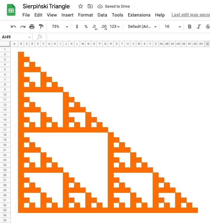
🔗 Get this example and others in the template at the bottom of this article.
It is named after the Polish mathematician Wacław Sierpiński and is also known as the Sierpiński gasket or Sierpiński sieve.
It has the property of being self-similar, meaning it looks the same at any magnification.
See Wikipedia for more on the Sierpiński triangle.
Continue reading How To Draw The Sierpiński Triangle In Google Sheets
The Cantor set is a special set of numbers lying between 0 and 1, with some fascinating properties.
It’s created by removing the middle third of a line segment and repeating ad infinitum with the remaining segments, as shown in this gif of the first 7 iterations:

The formulas used to create the data for the Cantor set in Google Sheets are interesting, so it’s worth exploring for that reason alone, even if you’re not interested in the underlying mathematical concepts.
But let’s begin by understanding the set in more detail…
The Cantor set was discovered in 1874 by Henry John Stephen Smith and subsequently named after German mathematician Georg Cantor.
The construction shown in this post is called the Cantor ternary set, built by removing the middle third of a line segment and repeating ad infinitum with the remaining segments.
It is sometimes known as Cantor dust on account of the dust of points that remain after repeatedly removing the middle thirds. (Cantor dust also refers to the multi-dimensional version of the Cantor set.)
The set has some fascinating, counter-intuitive properties:
Wow!
To be clear, the Cantor set is the set of numbers that remain after removing the middle third an infinite number of times. That’s hard to comprehend, let alone do in a Google Sheet 😉
But we can create a picture representation of the Cantor set by repeating the algorithm ten times, as shown in this tutorial:
Step 1:
In a blank sheet called “Data”, type the number “1” into cell A1.
Step 2:
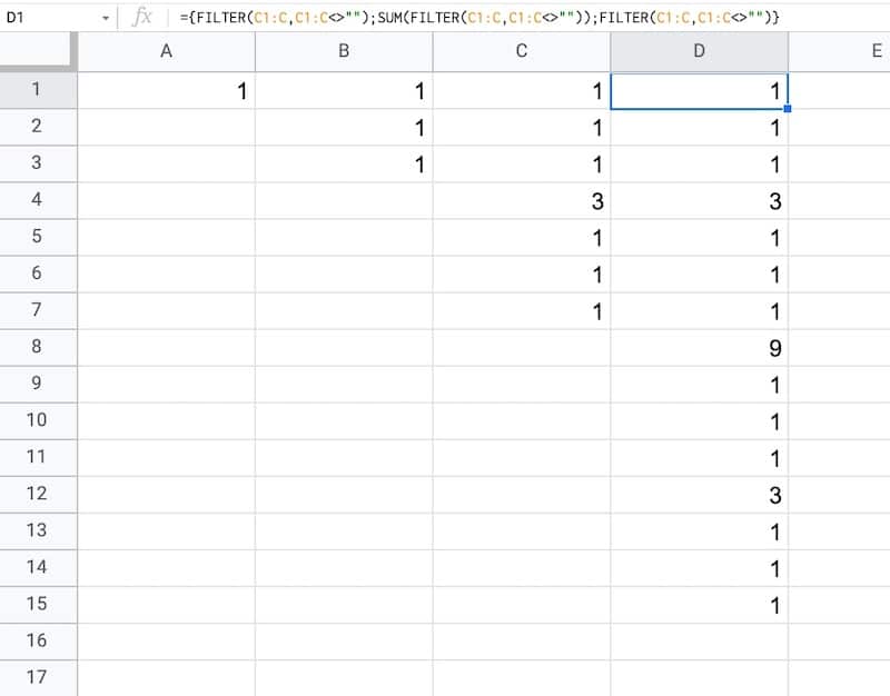
In cell B1, type this formula:
={ FILTER(A1:A,A1:A<>"") ;

SUM(FILTER(A1:A,A1:A<>"")) ;

FILTER(A1:A,A1:A<>"") }
Step 3:
Drag this across your sheet up to column J, which creates the data for the first 10 iterations.
Each formula references the column to the left. For example, the formula in cell D will reference column C.
Your data will look like this:
It combines array literals and the FILTER function.
Let’s break it down, using the onion framework.
The innermost formula is:
=FILTER(A1:A,A1:A<>"")This formula grabs all the data from column A and returns any non-blank entries, in this case just the value “1”.
Now we combine two of these together with array literals:
={ FILTER(A1:A,A1:A<>"") ;

FILTER(A1:A,A1:A<>"") }
Here the array literals { ... ; ... } stack these two ranges.
In this first example, it puts the number “1” with another “1” beneath it in column B.
Then we add a third FILTER and also SUM the middle FILTER range to create our final Cantor set algorithm:
={ FILTER(A1:A,A1:A<>"") ;

SUM(FILTER(A1:A,A1:A<>"")) ;

FILTER(A1:A,A1:A<>"") }
As we drag this formula to adjacent columns, the relative column references will change so that it always references the preceding column.
In column B, the output is:
1,1,1
Then in column C, we get:
1,1,1,3,1,1,1
And in column D:
1,1,1,3,1,1,1,9,1,1,1,3,1,1,1
etc.
This data is used to generate the correct gaps for the Cantor set.
We’ll use sparklines to draw the Cantor set in Google Sheets.
Step 4:
Create a new blank sheet and call it “Cantor Set”.
Step 5:
Next, create a label in column A to show what iteration we’re on.
Put this formula in cell A1 and copy down the column to row 10:
="Cantor Set "&ROW()This creates a string, e.g. “Cantor Set 1”, where the number is equal to the row number we’re on.
Step 6:
The next step is to dynamically generate the range reference. As we drag our formula down column B, we want this formula to travel across the row in the “Data” tab to get the correct data for this iteration of the Cantor set.
Start by generating the row number for each row with this formula in cell B1 and copy down the column:
=ROW()(I set up my sheet with the data in columns because it’s easier to create and read that way. But then I want the Cantor set in a column too, hence why I need to do this step.)
Step 7:
Use the row number to generate the corresponding column letter with this formula in cell C1 and copy down the column:
=ADDRESS(1,ROW(),4)This uses the ADDRESS function to return the cell reference as a string.
Step 8:
Remove the row number with this formula in cell D1 and copy down the column:
=SUBSTITUTE(ADDRESS(1,ROW(),4),"1","")Step 9:
Combine these two references to create an open-ended range reference for the correct column of data in the “Data” sheet.
Put this formula in cell E1 and copy down the column:
="'Data'!"&ADDRESS(1,ROW(),4)&":"&SUBSTITUTE(ADDRESS(1,ROW(),4),"1","")This returns range references e.g. 'Data'!A1:A
Step 10:
Put this formula in cell F1 and copy down the column:
=INDIRECT("'Data'!"&ADDRESS(1,ROW(),4)&":"&SUBSTITUTE(ADDRESS(1,ROW(),4),"1",""))This will show #REF! errors: “Array result was not expanded because it would overwrite data in…”
However, don’t worry, these are only temporary as we’ll dump this data into the sparkline formula next.
Step 11:
In column G, create a default sparkline formula:
=SPARKLINE(INDIRECT("'Data'!"&ADDRESS(1,ROW(),4)&":"&SUBSTITUTE(ADDRESS(1,ROW(),4),"1","")))This shows the default line chart (except for the first row where it shows a #N/A error).
Step 12:
In column H, convert the line chart sparkline to a bar chart sparkline by specifying the charttype in custom options:
=SPARKLINE(INDIRECT("'Data'!"&ADDRESS(1,ROW(),4)&":"&SUBSTITUTE(ADDRESS(1,ROW(),4),"1","")),{"charttype","bar"})Step 13 (optional):
Finally, in column I, change the colors to a simple black and white scheme, by specifying color1 and color2 inside the sparkline:
=SPARKLINE(INDIRECT("'Data'!"&ADDRESS(1,ROW(),4)&":"&SUBSTITUTE(ADDRESS(1,ROW(),4),"1","")),{"charttype","bar";"color1","black";"color2","white"})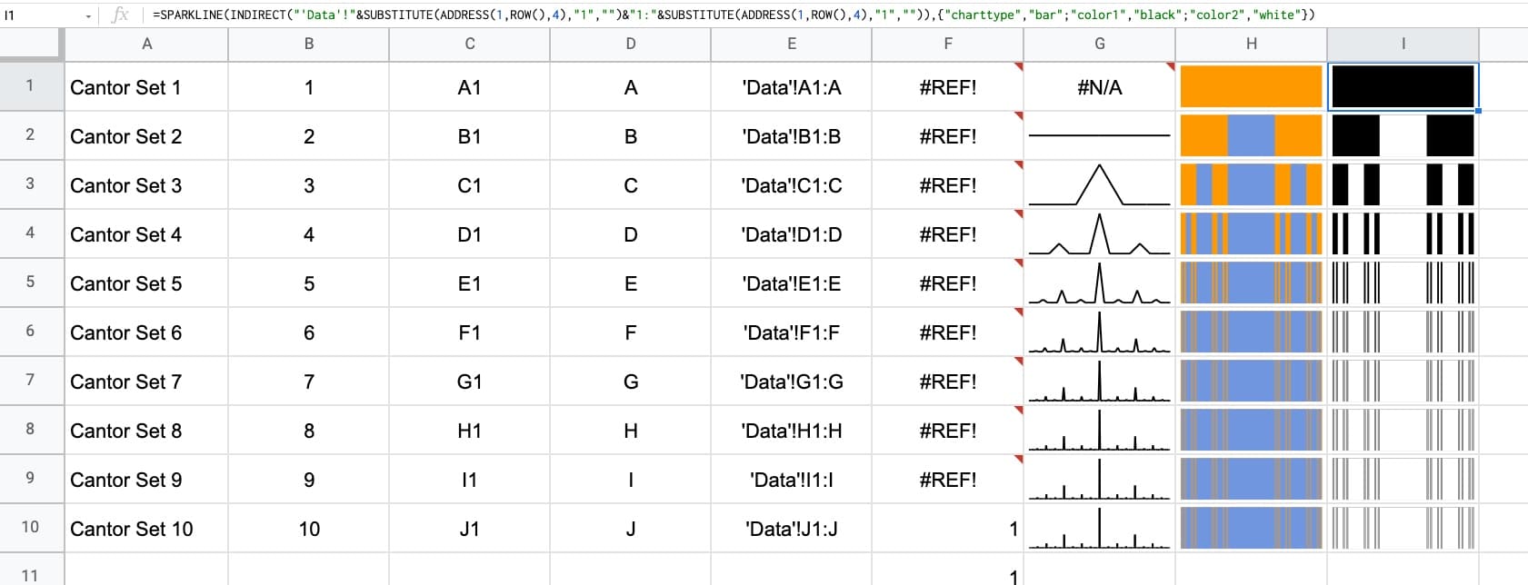
Feel free to delete any working columns once you have finished the formula showing the Cantor set.
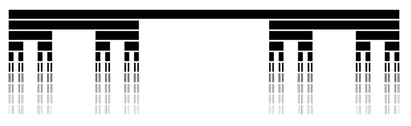
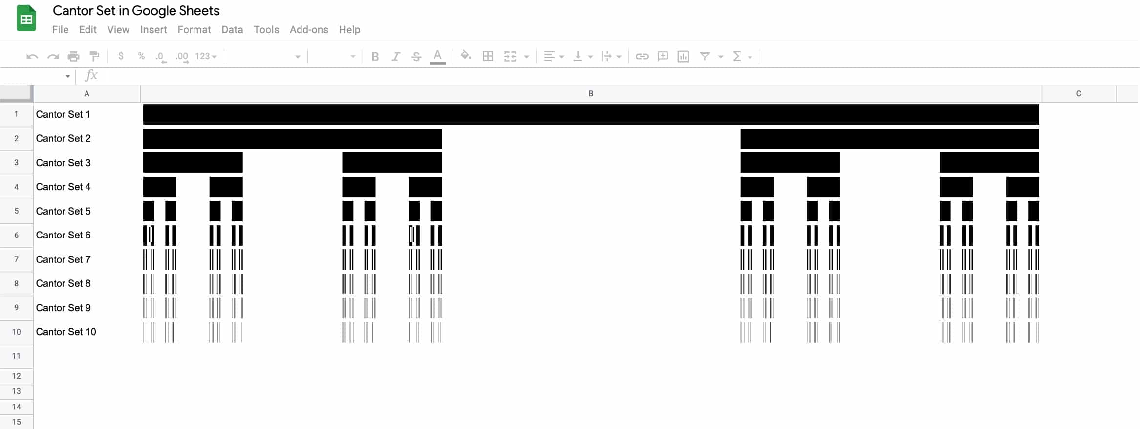
Here are the first 10 iterations of the algorithm to create the Cantor set:
Of course, this is a simplified representation of the Cantor set. It’s impossible to create the actual set in a Google Sheet since we can’t perform an infinite number of iterations.
You might enjoy my other mathematical Google Sheet posts:
PI Function in Google Sheets And Other Fun π Facts
Complex Numbers In Google Sheets
How To Draw The MandelBrot Set In Google Sheets, Using Only Formulas
The FACT Function in Google Sheets (And Why A Shuffled Deck of Cards Is Unique)
How To Draw The Sierpiński Triangle In Google Sheets
Exploring Population Growth And Chaos Theory With The Logistic Map, In Google Sheets
Let’s start with a mind-blowing fact, and then use the FACT function in Google Sheets to explain it.
Pick up a standard 52 card deck and give it a good shuffle.
The order of cards in a shuffled deck will be unique.
One that has likely never been seen before in the history of the universe and will likely never be seen again.
I’ll let that sink in.
Isn’t that mind-blowing?
Especially when you picture all the crazy casinos in Las Vegas.
Let’s understand why, and in the process learn about the FACT function and basic combinatorics (the study of counting in mathematics).
To keep things simple, suppose you only have 4 cards in your deck, the four aces.
You can create this deck in Google Sheets with the CHAR function:
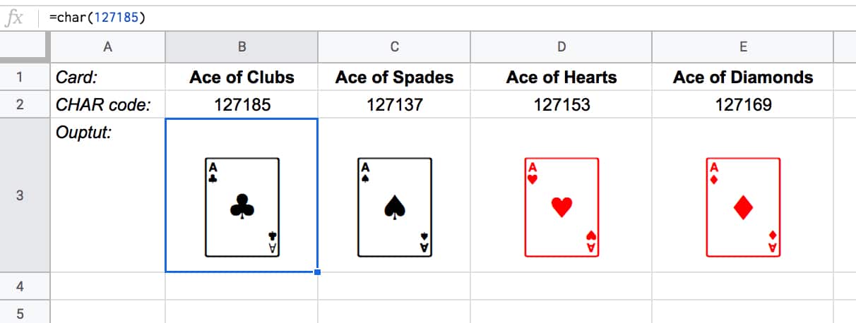
The formulas to create these four cards are:
Ace of Clubs:
=CHAR(127185)Ace of Spades:
=CHAR(127137)Ace of Hearts:
=CHAR(127153)Ace of Diamonds:
=CHAR(127169)Let’s see how many different combinations exist with just these four cards.
Pick one of them to start. You have a choice of four cards at this stage.
Once you’ve chosen the first one, you have three cards left, so there are 3 possible options for the second card choice.
When you’ve picked that second card, you have two cards left. So you have a choice of two for the third card.
The final card is the last remaining one.
So you have 4 choices * 3 choices * 2 choices * 1 choice = 4 * 3 * 2 * 1 = 24
There are 24 permutations (variations) with just 4 cards!
Visually, we can show this in our Google Sheet by displaying all the different combinations with the card images from above:
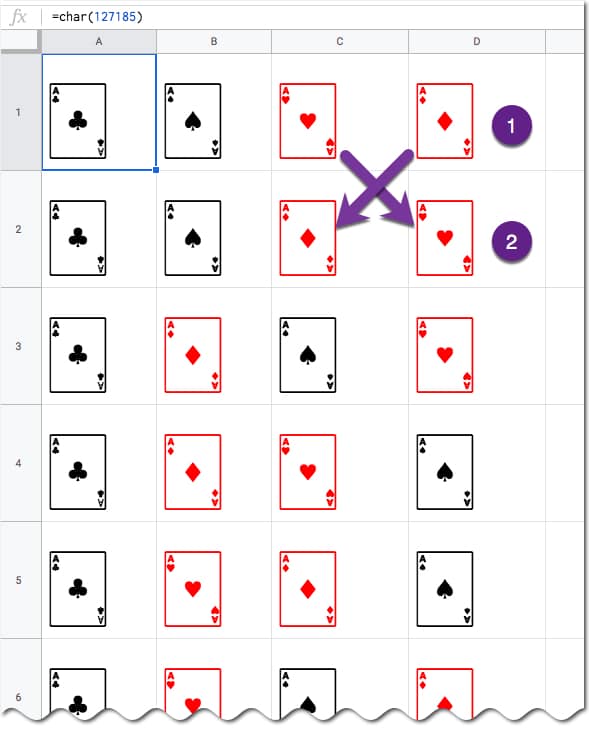
(I’ve just shown the first 6 rows for brevity.)
You can see for example, when moving from row 1 to row 2, we swapped the position of the two red suits: the Ace of Hearts and the Ace of Diamonds.
This time there are 5 choices for the first card, then 4, then 3, then 2, and finally 1.
So the number of permutations is 5 * 4 * 3 * 2 * 1 = 120
Already a lot more! I have not drawn this out in a Google Sheet and leave that as an optional exercise for you if you wish.
The FACT function in Google Sheets (see documentation) is a math function that returns the factorial of a given number. The factorial is the product of that number with all the numbers lower than it down to 1.
In other words, exactly what we’ve done above in the above calculations.
Four:
The 4 card deck formula is:
which gives an answer of 24 permutations.
Five:
The 5 card deck formula is:
which gives an answer of 120 permutations.
Six:
A 6 card deck is:
which gives an answer of 720 permutations.
Twelve:
A 12 card deck has 479,001,600 different ways of being shuffled:
(You’re more likely to win the Powerball lottery at 1 in 292 million odds than to get two matching shuffled decks of cards, even with just 12 cards!)
Fifty Two:
Keep going up to a full deck of 52 cards with the formula and it’s a staggeringly large number.
Type it into Google Sheets and you’ll see an answer of 8.07E+67, which is 8 followed by 67 zeros!
(This number notation is called scientific notation, where huge numbers are rounded to the first few digits multiplied by a 10 to the power of some number, 67 in this case.)
This answer is more than the number of stars in the universe (about 10 followed by 21 zeros).
Put another way if all 6 billion humans on earth began shuffling cards at 1 deck per minute every day of the year for millions of years, we still wouldn’t even be close to finding all possible combinations.