This post describes how I designed and ran an audience survey with over 1,700 responses, using Google Forms, Sheets, Apps Script, and ChatGPT. I’ll show you the entire process from end-to-end, including how I:
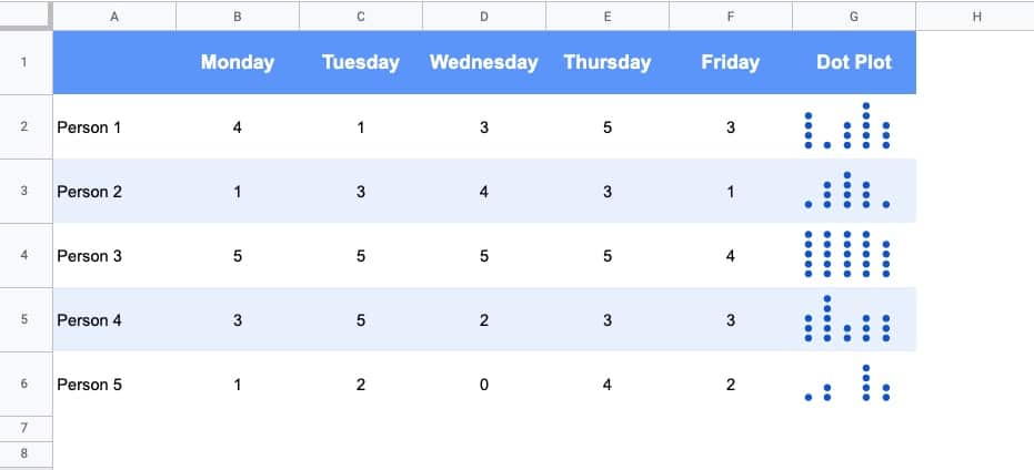
Dot plots are simple charts consisting of dots plotted on a simple scale, typically used to show small counts or distributions.
Dot plots are one of the simplest statistical charts, only suitable for small-sized data sets. They’re helpful for understanding the “shape” of your data by highlighting clusters, gaps, and outliers. (A histogram is better suited to showing the data distribution of larger datasets, e.g. > 30 datapoints.)
Here’s a table using dot plots to show the hypothetical number of meetings per day for these five employees:
How To Create Dot Plots In Google Sheets
You create dot plots in Google Sheets with formulas!
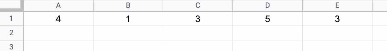
Suppose we have this data in row 1 of a Google Sheet, in cells A1 to E1:
Step 1:
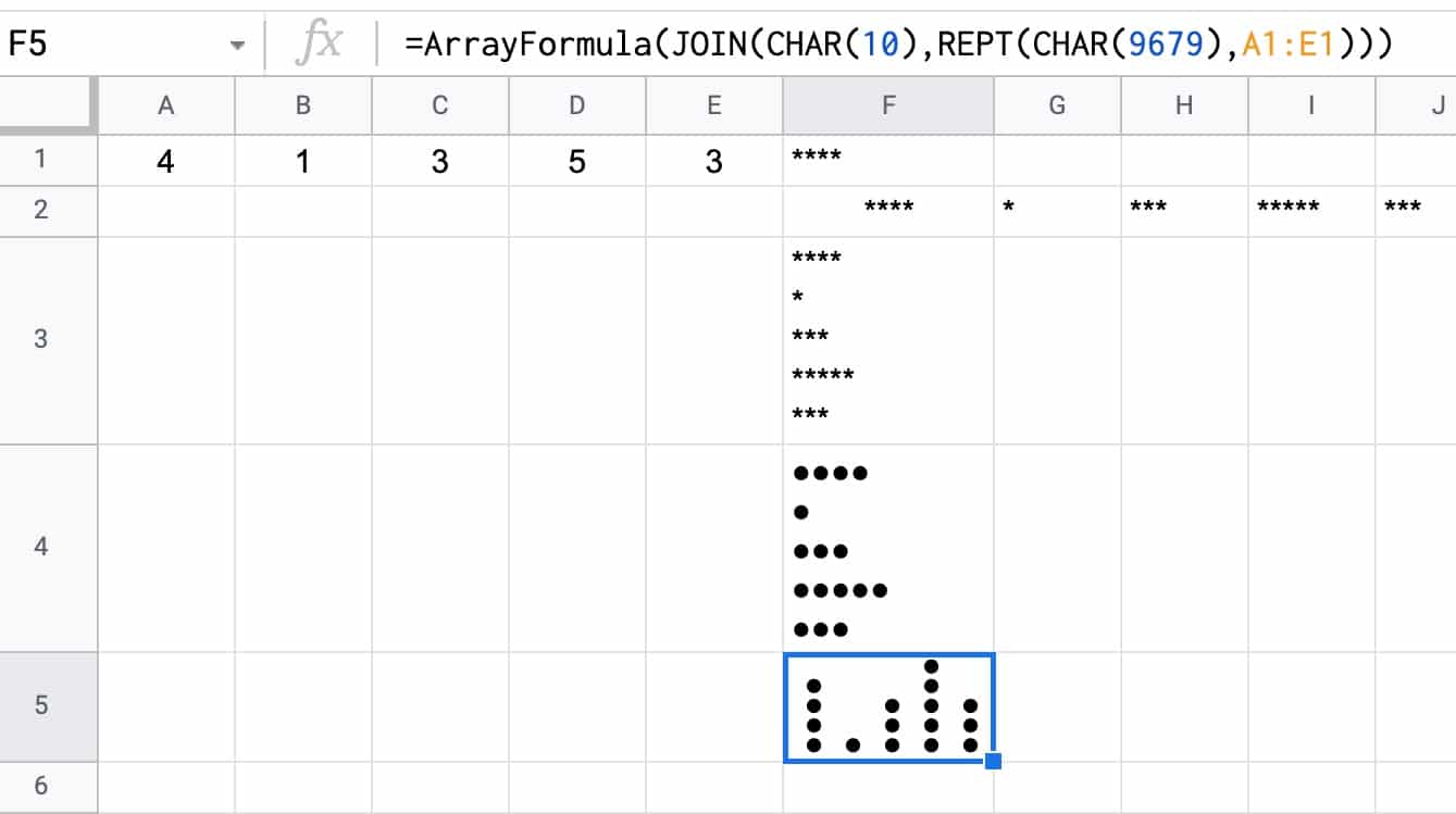
Create a basic REPT function next to the data, e.g. in cell F1:
It’s an array formula that takes an input of the five numbers in columns A to E.
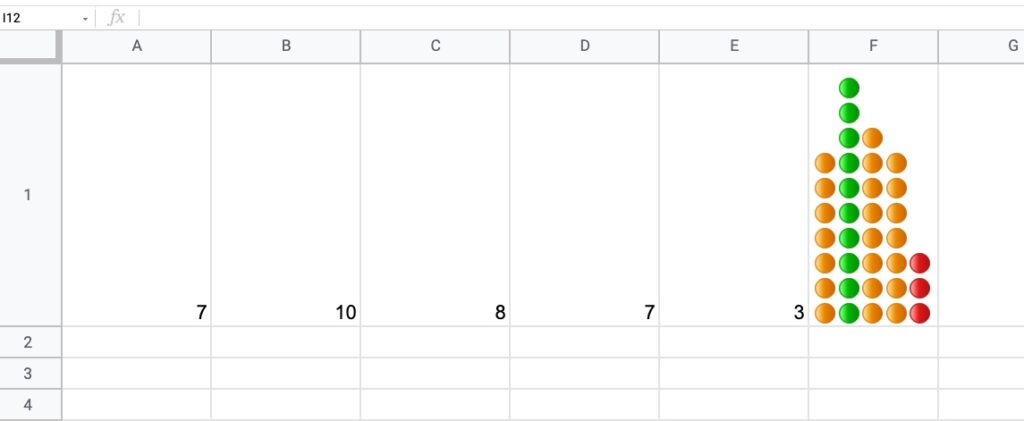
Inside the IFS function, the number (e.g. 7) is divided by the maximum number in the range (10 in this example) and compared to see if it’s bigger than the first threshold (0.85 in this example). If this is true, then the green dot is plotted, otherwise, the threshold is checked (0.5 in this example) If that’s true, then orange dot is used. If that is not true, then the red dot is used as the default.
The REPT function and the JOIN function perform the same way as step 3 above for the simpler single color example.
You can also replace the colored dots in this formula with their CHAR function equivalents, to keep it entirely formula driven:
The Cantor set is a special set of numbers lying between 0 and 1, with some fascinating properties.
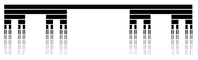
It’s created by removing the middle third of a line segment and repeating ad infinitum with the remaining segments, as shown in this gif of the first 7 iterations:
The formulas used to create the data for the Cantor set in Google Sheets are interesting, so it’s worth exploring for that reason alone, even if you’re not interested in the underlying mathematical concepts.
But let’s begin by understanding the set in more detail…
What Is The Cantor Set?
The Cantor set was discovered in 1874 by Henry John Stephen Smith and subsequently named after German mathematician Georg Cantor.
The construction shown in this post is called the Cantor ternary set, built by removing the middle third of a line segment and repeating ad infinitum with the remaining segments.
It is sometimes known as Cantor dust on account of the dust of points that remain after repeatedly removing the middle thirds. (Cantor dust also refers to the multi-dimensional version of the Cantor set.)
The set has some fascinating, counter-intuitive properties:
It is uncountable. That is, there are as many points left behind as there were to begin with.
It’s self-similar, meaning each subset looks like the whole set.
It’s fractal with a dimension that is not an integer.
It has an infinite number of points but a total length of 0.
Wow!
How To Draw The Cantor Set In Google Sheets
To be clear, the Cantor set is the set of numbers that remain after removing the middle third an infinite number of times. That’s hard to comprehend, let alone do in a Google Sheet 😉
But we can create a picture representation of the Cantor set by repeating the algorithm ten times, as shown in this tutorial:
Create The Data
Step 1:
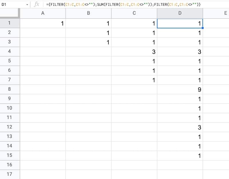
In a blank sheet called “Data”, type the number “1” into cell A1.
As we drag this formula to adjacent columns, the relative column references will change so that it always references the preceding column.
In column B, the output is:
1,1,1
Then in column C, we get:
1,1,1,3,1,1,1
And in column D:
1,1,1,3,1,1,1,9,1,1,1,3,1,1,1
etc.
This data is used to generate the correct gaps for the Cantor set.
Draw The Cantor Set
We’ll use sparklines to draw the Cantor set in Google Sheets.
Click to enlarge
Step 4:
Create a new blank sheet and call it “Cantor Set”.
Step 5:
Next, create a label in column A to show what iteration we’re on.
Put this formula in cell A1 and copy down the column to row 10:
="Cantor Set "&ROW()
This creates a string, e.g. “Cantor Set 1”, where the number is equal to the row number we’re on.
Step 6:
The next step is to dynamically generate the range reference. As we drag our formula down column B, we want this formula to travel across the row in the “Data” tab to get the correct data for this iteration of the Cantor set.
Start by generating the row number for each row with this formula in cell B1 and copy down the column:
=ROW()
(I set up my sheet with the data in columns because it’s easier to create and read that way. But then I want the Cantor set in a column too, hence why I need to do this step.)
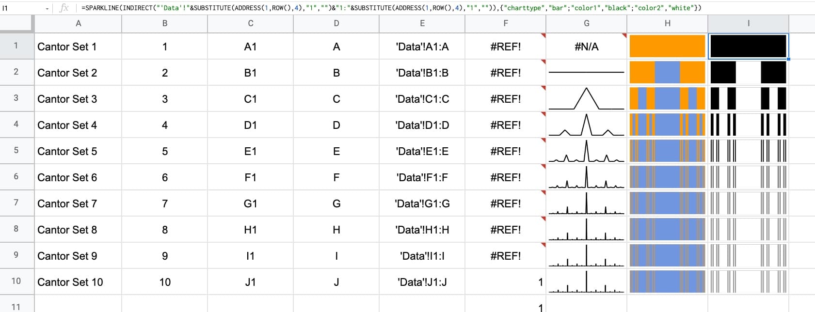
Step 7:
Use the row number to generate the corresponding column letter with this formula in cell C1 and copy down the column:
=ADDRESS(1,ROW(),4)
This uses the ADDRESS function to return the cell reference as a string.
Step 8:
Remove the row number with this formula in cell D1 and copy down the column:
=SUBSTITUTE(ADDRESS(1,ROW(),4),"1","")
Step 9:
Combine these two references to create an open-ended range reference for the correct column of data in the “Data” sheet.
Put this formula in cell E1 and copy down the column:
Feel free to delete any working columns once you have finished the formula showing the Cantor set.
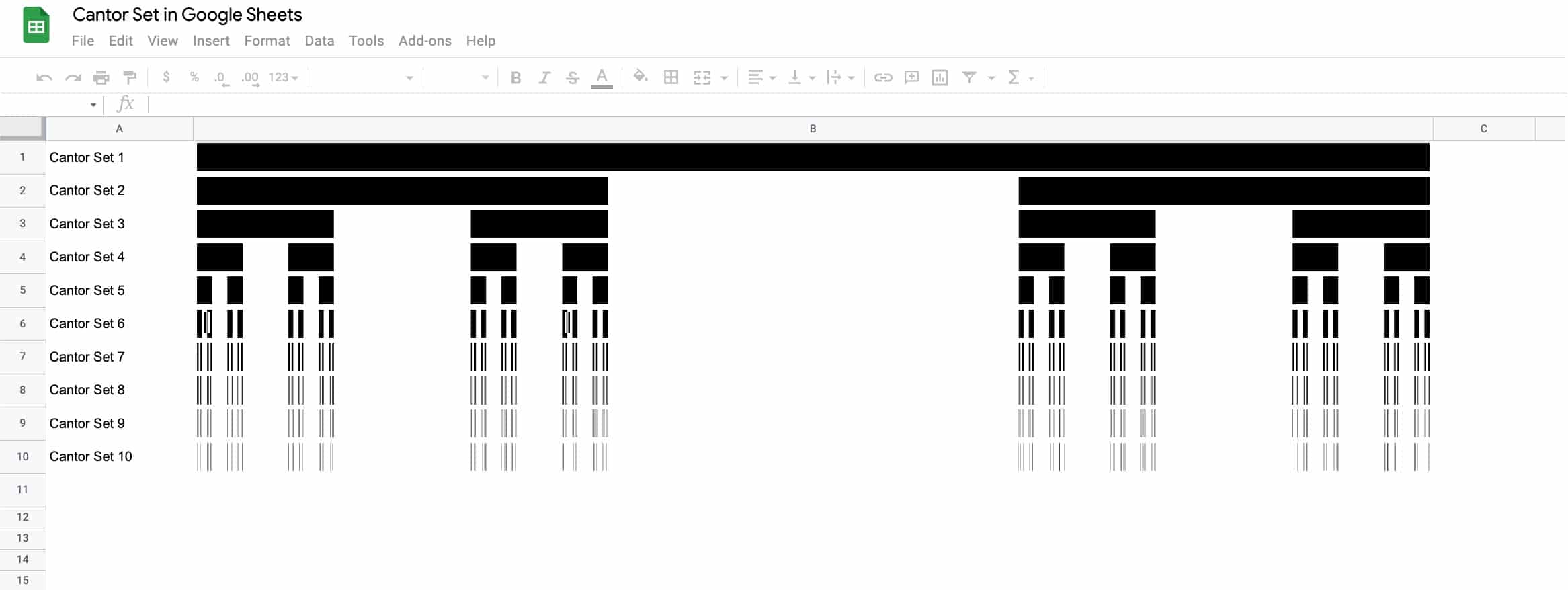
Finished Cantor Set In Google Sheets
Here are the first 10 iterations of the algorithm to create the Cantor set:
Click to enlarge
Of course, this is a simplified representation of the Cantor set. It’s impossible to create the actual set in a Google Sheet since we can’t perform an infinite number of iterations.
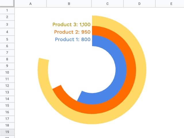
In this post, I’m going to show you how to create radial bar charts in Google Sheets.
They look great and grab your attention, which is important in this era of information overload.
But they should be used sparingly because they’re harder to read than a regular bar chart (because it’s harder to compare the length of the curved bars).
How To Create A Radial Bar Chart In Google Sheets
Let’s begin with the data.
In this example, we’ll create a radial bar chart in Google Sheets with 3 series.
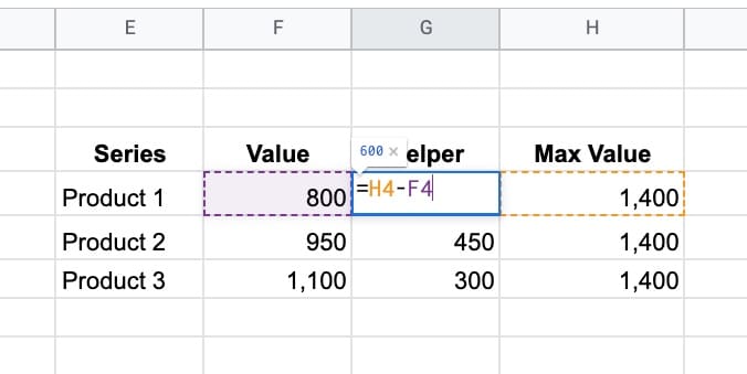
We need a column of values for these 3 series, for example, products with a number of units sold.
Next, we need some upper limit (max value) for our bars. This allows us to scale the bars properly.
Lastly, we need a helper column that calculates the difference between the max value and the actual value.
Here’s the data for the radial bar chart, in cells E3:H6:
Ok, I’m going to let you in on a little secret now…
This is not a single chart. No sir, it’s three charts overlaid on top of each other.
And yes, this means it takes three times as long to create!
Step 1: Create the inner circle
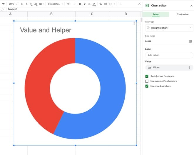
Highlight the first row of data but exclude the max value column. In the example dataset above, highlight E4:G4 and insert a chart.
Select a doughnut chart.
Under the Setup menu, make sure to check the “Switch rows/columns” checkbox, so your chart looks like this:
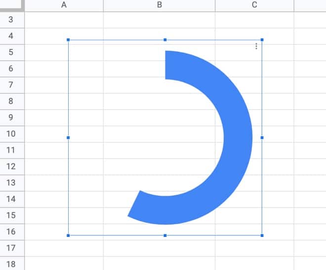
Under the customize menu of the chart tool, set the following conditions:
Background color: None
Chart border color: None
Donut hole size: 67%
Set Slice 2 color to none
Remove the chart title
Set the legend to none
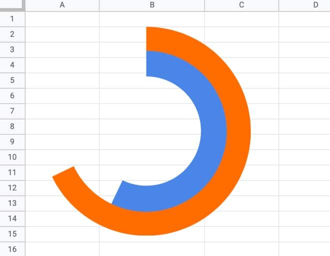
This is what the inner donut should look like:
Step 2: Create the middle circle
Repeat the steps above for the inner circle, but use the next row of data, choose a different color, and set the donut hole size to 77% (you may have to experiment with these percentages to line everything up at the end).
Drag the second donut chart on top of the first and line up the radial bars to get:
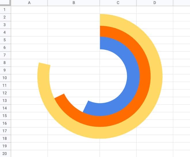
Step 3: Create the outer circle
Again, repeat the steps above from the inner circle to create a third donut chart, using the third row of data, a different color, and setting the donut hole size to 81% (again, this might need tweaking to line everything up).
Drag this third donut chart on top of the other two and you have a radial bar chart in Google Sheets!
Note on editing charts:
Since the charts are placed on top of each other, you’ll only be able to access the top chart to edit. You’ll have to move it to the side to access the chart underneath, and then move that one if you want to access the inner chart.
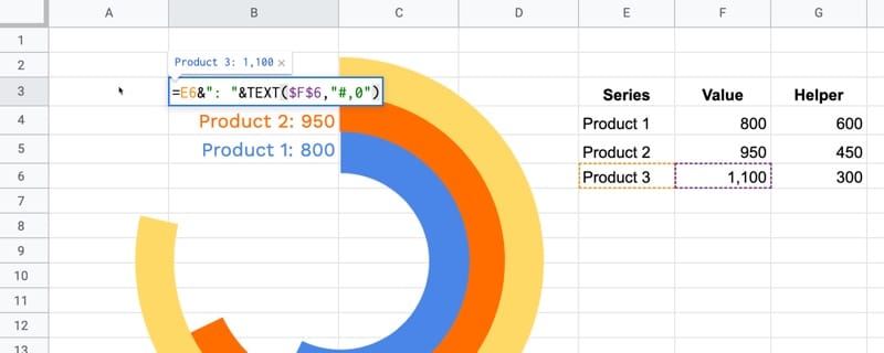
Step 4: Add the data labels
It gets messy to add the data labels to each chart through the chart editor, so I opted to create formulas to add my data labels into the cells next to each bar of the radial bar chart.
To access cells underneath the charts, click on a cell outside of the chart area and then use the arrow keys on your keyboard to reach the desired cell.
My friend Jeff Sauer, who founded Data Driven U to teach people data-driven marketing, contacted me recently about creating a radial bar chart for one of his workshops.
He is graciously sharing his report here, so you can see a radial bar chart with six rings:
This is a screenshot of his Google Sheet!
(If you’re looking for top draw digital marketing, then you should definitely check out Jeff’s site: DataDrivenU.com This is not an affiliate link, just a personal recommendation!)
You’ve probably also seen a radial bar chart in the wild with the Apple Watch Rings Chart!
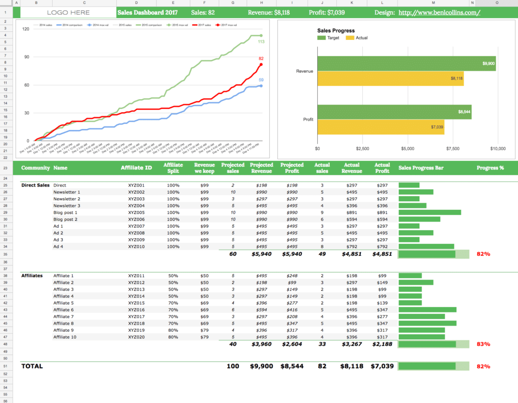
This post looks at how to make a line graph in Google Sheets, an advanced one with comparison lines and annotations, so the viewer can absorb the maximum amount of insight from a single chart.
For fun, I’ll also show you how to animate this line graph in Google Sheets.
The key to this line graph in Google Sheets is setting up the data table correctly, as this allows you to show an original data series (the grey lines in the animated GIF image), progress series lines (the colored lines in the animated GIF) and current data values (the data label on the series lines in the GIF).
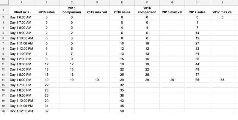
In this example, I have date and times as my row headings, as I’m measuring data across a 4-day period, and sales category figures as column headings, as follows:
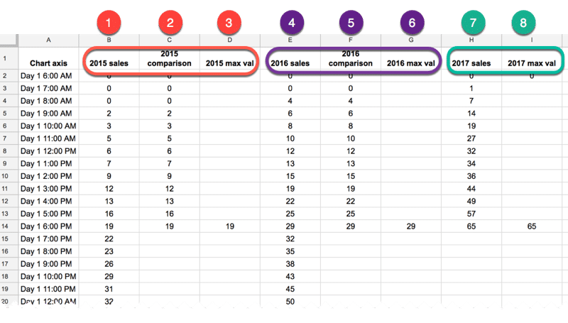
Red columns
The red column, labeled with 1 above, contains historic data from the 2015 sale.
Red column 2 is a copy of the same data but only showing the progress up to a specific point in time.
In red column 3, the following formula will create a copy of the last value in column 2, which is used to add a value label on the chart:
=IF(AND((C2+C3)=C2,C2<>0),C2,"")
Purple columns:
Purple columns 4,5 and 6 are exactly the same but for 2016 data. The formula in this case, in column 6, is:
=IF(AND((F2+F3)=F2,F2<>0),F2,"")
Green columns:
Data in green columns 7 and 8, is our current year data (2017), so in this case there is no column of historic data. The formula in column 8 for this example is:
=IF(AND((H2+H3)=H2,H2<>0),H2,"")
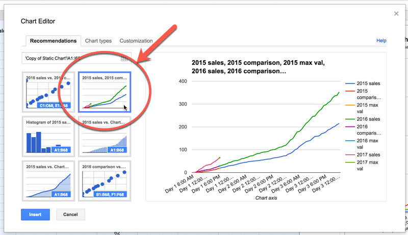
Creating the line graph in Google Sheets
Highlight your whole data table (Ctrl + A if you’re on a PC, or Cmd + A if you’re on a Mac) and select Insert > Chart from the menu.
In the Recommendations tab, you’ll see the line graph we’re after in the top-right of the selection. It shows the different lines and data points, so all that’s left to do is some formatting.
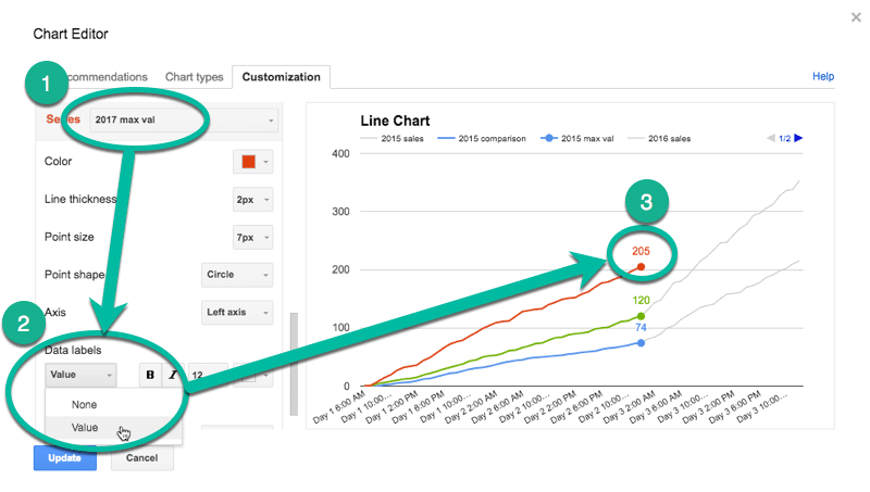
Format the series lines as follows:
For the historic data (columns 1 and 4 in the data table), make light grey and 1px thick
For the current data (columns 2, 5 and 7 in the data table), choose colors and make 2px thick
For the “max” values (columns 3, 6 and 8 in the data table), match the current data colors, make the data point 7px and add data label values (see steps 1, 2 and 3 in the image below)
This is the same technique I’ve written about in more detail in this post:
How about creating an animated version of this chart?
Oh, go on then.
When this script runs, it collects the historic data, then adds that data back to each new row after a 10 millisecond delay (achieved with the Utilities.sleep method and the SpreadsheetApp.flush method to apply all pending changes).
I don’t make any changes to the graph or create any fancy script to change it, I leave that up to the Google Chart Tool. It just does its best to keep up with the changing data, although as you can see from the GIF at the top of this post, it’s not silky smooth.
By the way, you can create and modify charts with Apps Script (see this waterfall chart example, or this funnel chart example) or with the Google Chart API (see this animated temperature chart). This may well be a better route to explore to get a smoother animation, but I haven’t tried yet…
Here’s the script:
function startTimedData() {
  var ss = SpreadsheetApp.getActive();
  var sheet = ss.getSheetByName('Animated Chart');
  var lastRow = sheet.getLastRow()-12;

  var data2015 = sheet.getRange(13,2,lastRow,1).getValues(); // historic data
  var data2016 = sheet.getRange(13,5,lastRow,1).getValues(); // historic data

  // new data that would be inputted into the sheet manually or from API
  var data2017 = [[1],[7],[14],[19],[27],[32],[34],[36],[44],[49],[57],[65],[72],[76],[79],[86],[92],[99],[104],[109],[111],[112],[120],[128],[130],
                  [132],[133],[140],[144],[149],[151],[152],[158],[162],[170],[177],[179],[184],[188],[194],[200],[205],[211],[216],[224],[232],[238],
                  [241],[246],[248],[252],[259],[266],[268],[276],[284],[291],[299],[300],[301],[306],[311],[315],[316],[323],[324]];

  for (var i = 0; i < data2015.length;i++) {
    outputData(data2015[i],data2016[i],data2017[i],i);
  }

}

function outputData(d1,d2,d3,i) {
  var ss = SpreadsheetApp.getActive();
  var sheet = ss.getSheetByName('Animated Chart');

  sheet.getRange(13+i,3).setValue(d1);
  sheet.getRange(13+i,6).setValue(d2);
  sheet.getRange(13+i,8).setValue(d3);
  Utilities.sleep(10);
  SpreadsheetApp.flush();
}

function clearData() {
  var ss = SpreadsheetApp.getActive();
  var sheet = ss.getSheetByName('Animated Chart');
  var lastRow = sheet.getLastRow()-12;

  sheet.getRange(13,3,lastRow,1).clear();
  sheet.getRange(13,6,lastRow,1).clear();
  sheet.getRange(13,8,lastRow,1).clear();

}
On lines 6 and 7, the script grabs the historic data for 2015 and 2016 respectively. For the contemporary 2017 data, I’ve created an array in my script to hold those values, since they don’t exist in my spreadsheet table.