Recursion in Google Sheets is now possible with the introduction of Named functions, LAMBDA functions, and LET functions. In this post, we’ll explore the concept of recursion and look at how to implement recursion in Google Sheets.
What is recursion?
In programming jargon, a recursive algorithm is a function that can call itself repeatedly until you stop it. Recursive functions allow you to loop through a problem in an elegant way, where updated parameters are passed between each call.
It’s critical to have a stop condition otherwise the recursion will continue forever (or, in practical terms, it’ll crash your program or give you an error message).
Recursion is a tricky concept to understand and implement.
Recursion in Google Sheets
There are two ways to implement recursion in Google Sheets: 1) with Named functions, and 2) with LET and LAMBDA functions.
We’ll explore both methods in this article, starting with a named function example:
Example 1: Reverse Word Order with Named Functions
Named functions in Google Sheets can call themselves recursively. You can include the function you’re defining as part of that function’s definition.
Let’s see an example from the Google’s documentation: how to reverse the order of words in a string.
Create a named function under the menu:
Data > Named functions
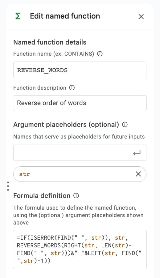
And define your named function REVERSE_WORDS thus:
=IF(ISERROR(FIND(" ", str)), str, REVERSE_WORDS(RIGHT(str, LEN(str)-FIND(" ", str)))&" "&LEFT(str, FIND(" ",str)-1))It looks like this in the named function sidebar:
In use, it’s a simple formula that takes a single string as an input and returns the string with the words in reverse order:
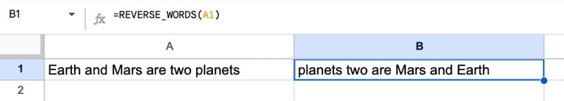
It works by moving the first word to the end of the string. It performs this same operation on the remaining portion of the original string on each iteration. When there are no spaces left in the remaining portion of the string (i.e. it’s on the final word and all the other words have been moved), it stops the recursion.
Named Functions Limitation
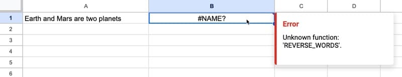
Named functions are incredibly powerful but they are only available in the spreadsheet where they are defined, or in copies of that spreadsheet, or spreadsheets that they have been imported into.
You can’t copy and paste a named function into a new spreadsheet. It won’t work because it doesn’t have the function’s underlying definition and you’ll see this error:
For the rest of this article, we’ll focus on recursive solutions that use the built-in functions, not the named functions. These solutions can be copied between sheets without this limitation described above.
LET and LAMBDA Together
Before we try a recursive formula with LET and LAMBDA, let’s see a simple example of how these two functions work together.
Try this LET formula in any cell of your Sheet:
=LET(

PLUSONE_,LAMBDA(x,x+1),

x,PLUSONE_(1),

x

)
The output is 2.
In the first line of the LET, we define a private function called PLUSONE_ that is a very simple LAMBDA function that adds 1 to the input.
Notice the underscore after the function name, a programming convention denoting a private function that’s only available inside its parent (in this case the LET function).
On the second line of the LET function, we define a variable x that calls the private PLUSONE_ function and passes in the argument 1 (or this could be a cell reference e.g. A1).
Finally, for the formula expression part of the LET, we simply print out the value of the variable x.
Obviously, this is a very complicated way of adding 1 to a number, but it shows you how we can define functions inside the LET and then use them in the formula expression. This is a very powerful way of working with formulas and is at the center of how the recursive examples work.
This sets us up nicely for looking at the recursive examples below.
Example 2: Linear Sum Example with LET and LAMBDA
Let’s see a simple recursion to calculate a linear sum. In this example, linear sum means add up all the integers up to and including an upper limit.
E.g. the linear sum of 10 is 1 + 2 + 3 + 4 + 5 + 6 + 7 + 8 + 9 + 10 = 55
In our Sheet, put a value in cell A1 (e.g. 10) and add this formula to cell B1:
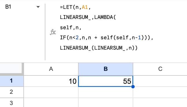
=LET(n,A1,

LINEARSUM_,LAMBDA(

self,n,

IF(n<2,n,n + self(self,n-1))),

LINEARSUM_(LINEARSUM_,n))
This formula calculates the total of all the integers up to and including the value in A1. In this case the answer is 55.
In the Sheet:
How does this formula work?
The best way to understand complex formulas is to peel them apart like onions, and work through each layer.
Here, the LET function defines the two variables: “n” and the recursive function “LINEARSUM_”.
LINEARSUM_ is defined as a LAMBDA function that contains a variable “self” that is used to reference itself (the recursion).
The heart of the LAMBDA is a simple IF statement that takes a variable “n”. Let’s understand it with actual numbers:
- On the first iteration, the LET function sets n = 10 (the value in cell A1)
- Since n (value 10) is greater than 2, it adds n to “self”, which is the recursive function call
- The recursive function — LINEARSUM_ — runs again but the value is now n-1, i.e. 9
- This loop continues with each successive value added to the accumulated total…
- …until n is less than 2, it returns the value of n. This is the stop case of the recursion.
Example 3: Linear Sum With the REDUCE Function
This is another recursive method, although the recursion is handled implicitly by the LAMBDA helper functions (in this case, the REDUCE function).
It’s a much shorter formula that is easier to understand than the LET/LAMBDA recursion example shown above.
=REDUCE(0,SEQUENCE(A1),LAMBDA(a,c,a+c))Here, a nested SEQUENCE function generates the array 1, 2, 3, …, 10, which is passed as an array into the REDUCE function.
The initial value is 0 and the LAMBDA simply adds the accumulated value (“a”) to the current value (“c”) at each iteration. For the first iteration, a = 0 and c = 1, which add together to give 1. For the second iteration, now a = 1 and c = 2, so the new accumulated value is 3, etc.
Example 4: Fibonacci Sequence
This example comes from this excellent Stack Overflow post on recursion in Google Sheets. Hat tip to the author!
To find a specific digit of the Fibonacci sequence, we use this recursive formula:
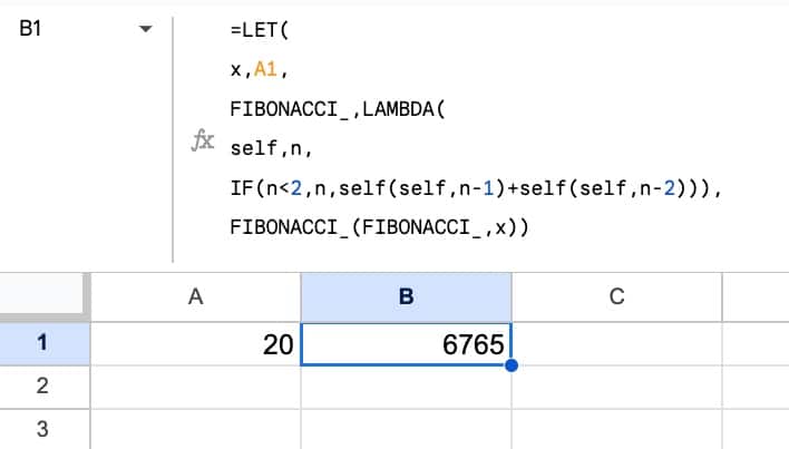
=LET(

x,A1,

FIBONACCI_,LAMBDA(

self,n,

IF(n<2,n,self(self,n-1)+self(self,n-2))),

FIBONACCI_(FIBONACCI_,x))
In our Sheet, this gives the correct answer of 6,765 with a starting value of 20:
To understand how this is working, let’s strip out the guts of the LAMBDA function and focus on the LET and recursion elements:
=LET(

x,A1,

FIBONACCI_,LAMBDA( ... ),

FIBONACCI_(FIBONACCI_,x))
The LET function defines two variables:
- x, which takes the value in cell A1, and
- FIBONACCI_, which is defined inside the LAMBDA
Following the two variables is the formula description part of our LET function, where we call the private function:
FIBONACCI_(FIBONACCI_,x)FIBONACCI_ and x are passed as arguments into the LAMBDA function (into the parameters “self” and “n” respectively).
Quick clarification: parameters are the placeholder variables in the function definition, whereas arguments are the actual values passed into the function.
Now, back to the LAMBDA part of the formula:
LAMBDA(

self,n,

IF(n<2,n,self(self,n-1)+self(self,n-2)))
The “self” and “n” are the parameters of the LAMBDA function.
Much like the IF function in the linear sum example above, the heart of the LAMBDA is an IF statement that includes the stop case (when n < 2). With each loop, it calls itself with n-1 and n-2 values to calculate the two numbers prior that are added together for the Fibonacci sequence.
The output of the formula is the accumulated value, which is the Fibonacci sequence value for that specific digit.
Calculation Limit
The upper limit for this formula is 24 digits.
Beyond this we hit the calculation limits of Google Sheets and see this error message: “Calculation limit was reached while trying to compute this formula.”.
Now, let’s convert this to an array formula to show the full Fibonacci sequence.
Fibonacci Array Formula Extension
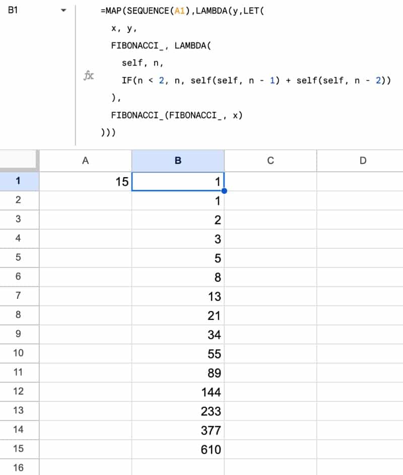
We turn this into an array formula by wrapping it with the MAP function, so that it outputs the full Fibonacci sequence up to a given number:
=MAP(SEQUENCE(A1),LAMBDA(y,LET(

  x, y,

  FIBONACCI_, LAMBDA(

    self, n,

    IF(n < 2, n, self(self, n - 1) + self(self, n - 2))
  ),
  FIBONACCI_(FIBONACCI_, x))))
A SEQUENCE function turns the value in A1 into an array 1,2,3,4, etc. Then the MAP function maps the values in that array into their respective Fibonacci digits, calculated by the inner recursive formula.
The output of this MAP formula is the full Fibonacci sequence up to the specified limit:
The upper calculation limit with this array version is 22 digits of the Fibonacci sequence.
Non-LAMBDA Alternative
See also this excellent implementation of the Fibonacci sequence from developer Max Makhrov, using only the SEQUENCE and INDEX functions. This has a much higher upper limit than the recursive method. Hat tip to you Max!
Example 5: Sieve of Eratosthenes
The Sieve of Eratosthenes is an ancient algorithm for finding all the prime numbers up to a given limit.
The Google Sheets formula for this algorithm is:
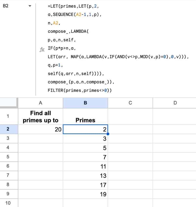
=LET(primes,LET(p,2,

a,SEQUENCE(A2-1,1,p),

n,A2,

COMPOSE_,LAMBDA(

p,a,n,self,

IF(p*p>n,a,

LET(arr, MAP(a,LAMBDA(v,IF(AND(v<>p,MOD(v,p)=0),0,v))),

q,p+1,

self(q,arr,n,self)))),

COMPOSE_(p,a,n,COMPOSE_)),

FILTER(primes,primes<>0))
It's a translation of a JavaScript algorithm (#7 in the this list).
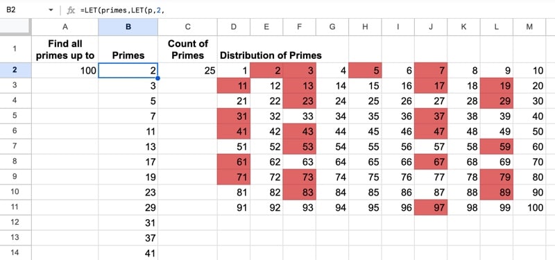
This formula outputs a list of prime numbers under a given limit:
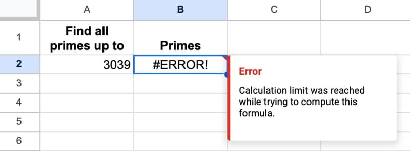
The upper limit for this recursion formula is 3038. If we try to find all primes up to 3,039 then we get this error message: "Calculation limit was reached while trying to compute this formula."
Understanding the Primes
With a list of the prime numbers, we can do a few other checks.
We can easily count the number of primes in our population, which serves as a check. Although it doesn't confirm our list is correct, it would indicate if we had an error.
The formula is very simple count of the primes in column B:
=COUNT(B2:B)We can also visualize the distribution of the primes, which is interesting to see.
First, create an array of numbers in 10 columns with this formula:
=SEQUENCE(A2/10,10)Then apply conditional formatting to the range D2:M1000 with this custom formula format rule:
=VLOOKUP(D2,$B:$B,1,FALSE)>0The conditional formatting sidebar looks like this:
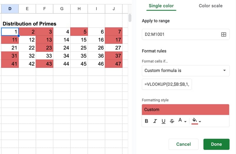
This will highlight all of the prime numbers as follows:
Recursion in Google Sheets Template
🔗 Click here to open a view-only copy >>
Feel free to make a copy: File > Make a copy…
If you can’t access the template, it might be because of your organization’s Google Workspace settings.
In this case, right-click the link to open it in an Incognito window to view it.
Brilliant, Ben. Thanks for introducing me to this. It’s certainly challenging.
One very tiny detail. The SEQUENCE function is one row short – try it with 3038 in cell A2 and you will see what I mean. I changed it to SEQUENCE((A2/10)+1,10) to display the last prime (3037).
I was wondering why you would reach the calculation limit at such a low number for the Fibinocci sequence, but then I realized two things. First, your recursion is doubling on each loop because it called the inner recursive function twice in the same statement. Second, I think you’re going in the wrong direction with that recursion. If I asked you to give me the 6th number, would you say 6th = 5th + 4th, and the 5th = 4th + 3rd and 4th = 3rd + 2nd, and so on. That means 6th = (4th + 3rd) + (3rd + 2nd). Not done yet. Still have to recurse those. 6th = ((3rd + 2nd) + (2nd + 1st)) + ((2nd + 1st) + 2nd) = (((2nd + 1st) + 2nd) + (2nd + 1st)) + ((2nd + 1st) + 2nd) = 8.
No, you would go the other direction, building up to the 6th number. All you need to know at each step are the previous two number in the sequence and what step you’re at. We can rewrite your function like this:
=LET(
x,A1,
FIBONACCI_,LAMBDA(
self,n,prev,cur,
IF(n<2,cur,self(self,n-1,cur,prev+cur))),
FIBONACCI_(FIBONACCI_,x,0,1))
We are still keeping track of the counter to know when to terminate, but if we haven't reached that point, we call the recursive function, this time passing current number (will become the "prev") and our last number plus the current number (will become the next "cur").
I think sheets reaches it's precision limit before reaching its calculation limit using this approach.
As always, enjoying your posts.
-Shay
One thing worth noting here is that you have to go through a bit of a contrivance to create recursion with Lambda, due to a strange manner of the way it seems to bind names.
The much more traditional – and straightforward – way to define LINEARSUM via lambda would have been:
=LET(n,A1,
LINEARSUM_,LAMBDA(n,
IF(n<2,n,n + LINEARSUM_(n-1))),
LINEARSUM_(n))
without the need to pass in the lambda itself. But this fails because the inner call to LINEARSUM_ is unable to resolve the name LINEARSUM. It gives a #NAME? error.
This really needs to be fixed. The LET is not making the name LINEARSUM available until the value itself is fully defined. But it doesn't need the definition at that point, only the name. It's declaration should be sufficient to call it. It's lazy evaluation, anyway, after all.
This deficiency really needs to be fixed, it makes such inner recursion much more cumbersome. After all, one of the places you would use lamba recursion is itself *inside* a Named Function. The outer Named Function takes ALL of the parameters that are needed for all the work, but the recursion portions of computation might be performed by a smaller lambda inside, one which doesn't need all of those variables parameterized for each call -where the other values passed into the named function are constant during the calculation.
Ironically, Named Functions do not themselves accept other functions or lambdas as arguments. The parameter named cannot be called as a function. Go figure. Another deficiency/inconsistency that needs to be fixed.