This Formula Challenge originally appeared as Tip #131 of my weekly Google Sheets Tips newsletter, on 21 December 2020.
Sign up here so you don’t miss out on future Formula Challenges:
Find all the Formula Challenges archived here.
The Challenge: Merge Columns With Single Range Reference
Question: How can you merge n number of columns and get the unique values, without typing each one out?
In other words, can you create a single formula that gives the same output as this one:
=SORT( UNIQUE( {A:A;B:B;C:C;...;XX:XX} )) but without having to write out A:A, B:B, C:C, D:D etc. and instead just write A:XX as in the input?
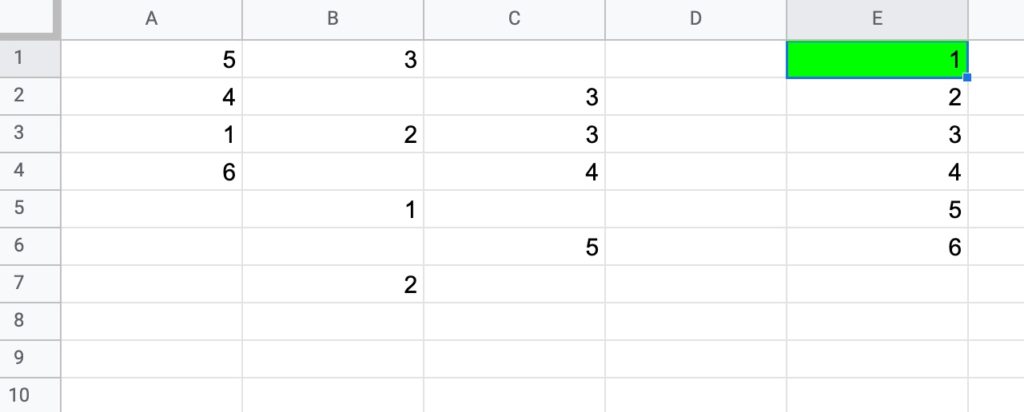
Use this simple dataset example, where your formula will be in cell E1 (in green):
Your answer should:
- be a formula in a single cell
- work with the input range in the form A:XX (e.g. A:C in this example)
- work with numbers and/or text values
- return only the unique values, in an ascending order in a SINGLE COLUMN.
Solutions To Sort A Column By Last Name
I received 67 replies to this formula challenge with two different methods for solving it. Congratulations to everyone who took part!
I learnt so much from the different replies, many of which proffered a shorter and more elegant second solution than my own original formula.
Here I present the two solutions.
There’s a lot to learn by looking through them.
1. FLATTEN method
=SORT(UNIQUE(FLATTEN(A:C)))The formula uses the FLATTEN function to collect data from the input ranges into a single column before the UNIQUE function selects the unique ones before they are finally sorted.
Note 1: you can have multiple inputs (arguments) to the FLATTEN function. Data is ordered by the order of the inputs, then row and then column.
Note 2: at the moment the FLATTEN function doesn’t show up in the auto-complete when you start typing it out. You can still use it, but you’ll have to type it out fully yourself.
Thanks to the handful of you that shared this neat solution with me. Great work!
2. TEXTJOIN method
Join all the values in A:C with TEXTJOIN, using a unique character as the delimiter (in this case, the King and Queen chess pieces!)
You want to use an identifier that is not in columns A to C.
=TEXTJOIN("♔♕",TRUE,A:C)Split on this unique delimiter using the SPLIT function:
=SPLIT(TEXTJOIN("♔♕",TRUE,A:C),"♔♕")Use the TRANSPOSE function to switch to a column, select the unique values only and finally wrap with a sort function to get the result:
=SORT(UNIQUE(TRANSPOSE(SPLIT(TEXTJOIN("♔♕",TRUE,A:C),"♔♕"))))There we go!
Two brilliant solutions to an interesting formula challenge.
Please leave comments if you have anything you wish to add.
And don’t forget to sign up to my Google Sheets Tips newsletter so you don’t miss future formula challenges!
One issue I have with your first solution is that it also includes a blank cell after all of the digits as part of the returned array.
A better alternative would be TOCOL, since it can easily filter out the blank cells.
=SORT(UNIQUE(TOCOL(A:C, 1)))
Nice! Thanks for sharing, Shay. This post predates the introduction of TOCOL, so it’s nice to see these new functions can produce a better answer.