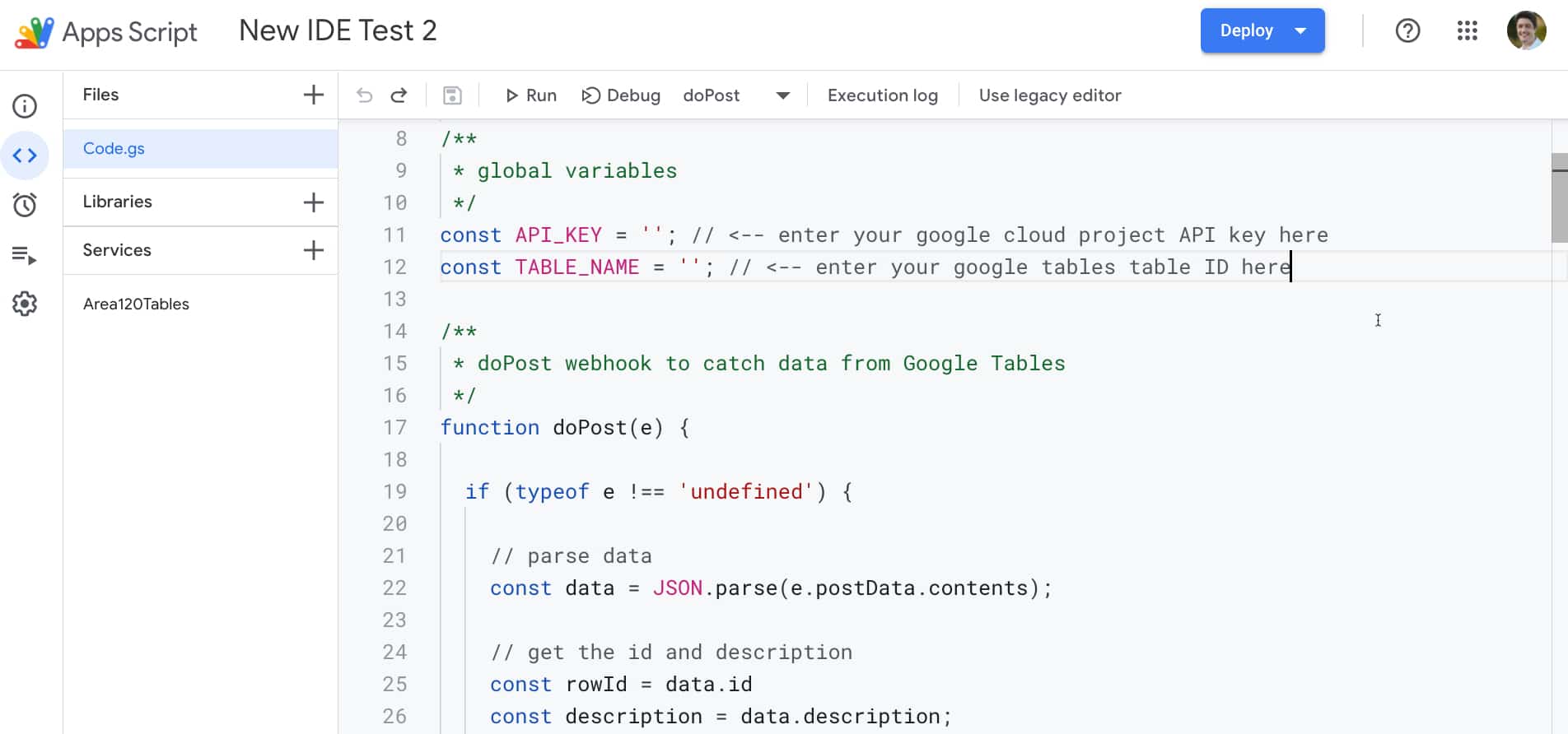
If you have a Nest thermostat at home, you can access it from your Google Sheet by using Google Apps Script to connect to the Smart Device Management API.
It means you can do some cool stuff like build a virtual, working Nest thermostat in your Google Sheet:
💡 Learn moreLearn how to write Apps Script and turbocharge your Google Workspace experience with the new Beginner Apps Script course
Google Sheets Macros are small programs you create inside of Google Sheets without needing to write any code.
They’re used to automate repeatable tasks. They work by recording your actions as you do something and saving these actions as a “recipe” that you can re-use again with a single click.
For example, you might apply the same formatting to your charts and tables. It’s tedious to do this manually each time. Instead you record a macro to apply the formatting at the click of a button.
In this article, you’ll learn how to use them, discover their limitations and also see how they’re a great segue into the wonderful world of Apps Script coding!
Think of a typical day at work with Google Sheets open. There are probably some tasks you perform repeatedly, such as formatting reports to look a certain way, or adding the same chart to new sales data, or creating that special formula unique to your business.
They all take time, right?
They’re repetitive. Boring too probably. You’re just going through the same motions as yesterday, or last week, or last month. And anything that’s repetitive is a great contender for automating.
This is where Google Sheets macros come in, and this is how they work:
Click a button to start recording a macro
Do your stuff
Click the button to stop recording the macro
Redo the process whenever you want at the click of a button
There’s the obvious reason that macros in Google Sheets can save you heaps of time, allowing you to focus on higher value activity.
But there’s a host of other less obvious reasons like: avoiding mistakes, ensuring consistency in your work, decreased boredom at work (corollary: increased motivation!) and lastly, they’re a great doorway into the wonderful world of Apps Script coding, where you can really turbocharge your spreadsheets and Google Workspace work.
Let’s run through the process of creating a super basic macro, in steps:
1) Open a new Google Sheet (pro-tip 1: type sheets.new into your browser to create a new Sheet instantly, or pro-tip 2: in your Drive folder hit Shift + s to create a new Sheet in that folder instantly).
Type some words in cell A1.
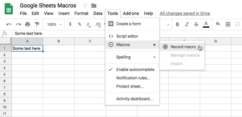
2) Go to the macro menu: Tools > Macros > Record macro
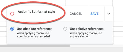
3) You have a choice between Absolute or Relative references. For this first example, let’s choose relative references:
Absolute references apply the formatting to the same range of cells each time (if you select A1:D10 for example, it’ll always apply the macro to these cells). It’s useful if you want to apply steps to a new batch of data each time, and it’s in the same range location each time.
Relative references apply the formatting based on where your cursor is (if you record your macro applied to cell A1, but then re-run the macro when you’ve selected cell D5, the macro steps will be applied to D5 now). It’s useful for things like formulas that you want to apply to different cells.
4) Apply some formatting to the text in cell A1 (e.g. make it bold, make it bigger, change the color, etc.). You’ll notice the macro recorder logging each step:
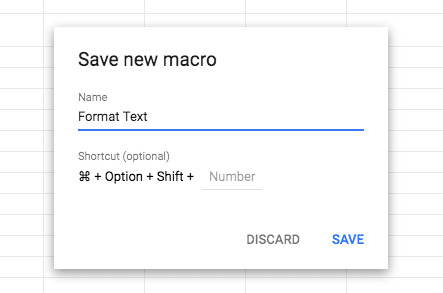
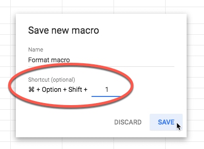
5) When you’ve finished, click SAVE and give your Macro a name:
(You can also add a shortcut key to allow quick access to run your macro in the future.)
Click SAVE again and Google Sheets will save your macro.
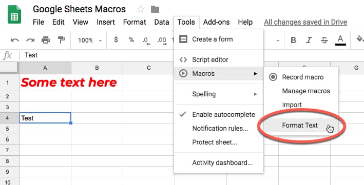
6) Your macro is now available to use and is accessed through the Tools > Macros menu:
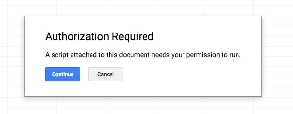
7) The first time you run the macro, you’ll be prompted to grant it permission to run. This is a security measure to ensure you’re happy to run the code in the background. Since you’ve created it, it’s safe to proceed.
First, you’ll click Continue on the Authorization popup:
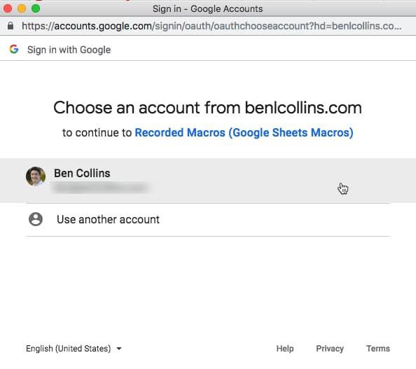
Then select your Google account:
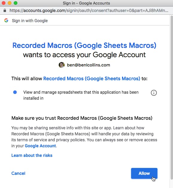
Finally, review the permissions, and click Allow:
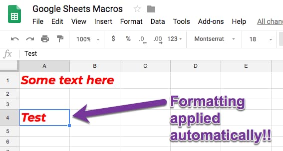
8) The macro then runs and repeats the actions you recorded on the new cell you’ve selected!
You’ll see the following yellow status messages flash across the top of your Google Sheet:
and then you’ll see the result:
Woohoo!
Congratulations on your first Google Sheets macro! You see, it was easy!
Here’s a quick GIF showing the macro recording process in full:
This is an optional feature when you save your macro in Google Sheets. They can also be added later via the Tools > Macros > Manage macros menu.
Shortcuts allow you to run your macros by pressing the specific combination of keys you’ve set, which saves you further time by not having to click through the menus.
Any macro shortcut keys must be unique and you’re limited to a maximum of 10 macro shortcut keys per Google Sheet.
In the above example, I could run this macro by pressing:
⌘ + option + shift + 1
keys at the same time (takes practice ?). Will be a different key combo on PC/Chromebooks.
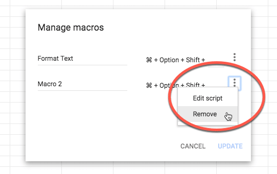
4.2 Deleting macros
You can remove Google Sheets macros from your Sheet through the manage macros menu: Tools > Macros > Manage macros
Under the list of your macros, find the one you want to delete. Click the three vertical dots on right side of macro and then choose Remove macro:
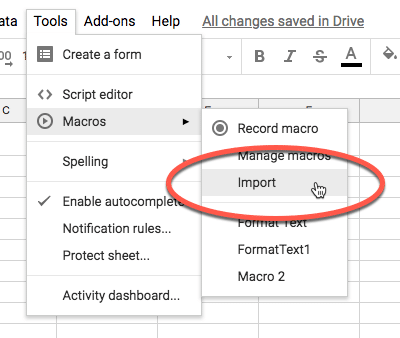
4.3 Importing other macros
Lastly, you can add any functions you’ve created in your Apps Script file to the Macro menu, so you can run them without having to go to the script editor window. This is a more advanced option for users who are more comfortable with writing Apps Script code.
This option is only available if you have functions in your Apps Script file that are not already in the macro menu. Otherwise it will be greyed out.
Use the minimum number of actions you can when you record your macros to keep them as performant as possible.
For macros that make changes to a single cell, you can apply those same changes to a range of cells by highlighting the range first and then running the macro. So it’s often not necessary to highlight entire ranges when you’re recording your macros.
Macros are bound to the Google Sheet in which they’re created and can’t be used outside of that Sheet. Similarly, macros written in standalone Apps Script files are simply ignored.
Macros are not available for other Google Workspace tools like Google Docs, Slides, etc. (At least, not yet.)
You can’t distribute macros as libraries or define them in Sheets Add-ons. I hope the distribution of macros is improved in the future, so you can create a catalog of macros that is available across any Sheets in your Drive folder.
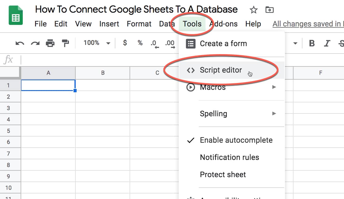
If you want to take a look at this code, you can see it by opening the script editor (Tools > Script editor or Tools > Macros > Manage macros).
You’ll see an Apps Script file with code similar to this:
/** @OnlyCurrentDoc */

function FormatText() {
  var spreadsheet = SpreadsheetApp.getActive();
  spreadsheet.getActiveRangeList().setFontWeight('bold')
  .setFontStyle('italic')
  .setFontColor('#ff0000')
  .setFontSize(18)
  .setFontFamily('Montserrat');
};
Essentially, this code grabs the spreadsheet and then grabs the active range of cells I’ve selected.
The macro then makes this selection bold (line 5), italic (line 6), red (line 7, specified as a hex color), font size 18 (line 8), and finally changes the font family to Montserrat (line 9).
The video at the top of this page goes into a lot more detail about this Apps Script, what it means and how to modify it.
Macros in Google Sheets are a great first step into the world of Apps Script, so I’d encourage you to open up the editor for your different macros and check out what they look like.
(In case you’re wondering, the line /** @OnlyCurrentDoc */ ensures that the authorization procedure only asks for access to the current file where your macro lives.)
Record the steps as you format your reporting tables, so that you can quickly apply those same formatting steps to other tables. You’ll want to use Relative references so that you can apply the formatting wherever your table range is (if you used absolute then it will always apply the formatting to the same range of cells).
Check out the video at the top of the page to see this example in detail, including how to modify the Apps Script code to adjust for different sized tables.
8.2 Creating charts
If you find yourself creating the same chart over and over, say for new datasets each week, then maybe it’s time to encapsulate that in a macro.
Record your steps as you create the chart your first time so you have it for future use.
The video at the top of the page shows an example in detail.
The following macros are intended to be copied into your Script Editor and then imported to the macro menu and run from there.
8.3 Convert all formulas to values on current Sheet
Open your script editor (Tools > Script editor). Copy and paste the following code onto a new line:
// convert all formulas to values in the active sheet
function formulasToValuesActiveSheet() {
  var sheet = SpreadsheetApp.getActiveSheet();
  var range = sheet.getDataRange();
  range.copyValuesToRange(sheet, 1, range.getLastColumn(), 1, range.getLastRow());
};
Back in your Google Sheet, use the Macro Import option to import this function as a macro.
When you run it, it will convert any formulas in the current sheet to values.
8.4 Convert all formulas to values in entire Google Sheet
Open your script editor (Tools > Script editor). Copy and paste the following code onto a new line:
// convert all formulas to values in every sheet of the Google Sheet
function formulasToValuesGlobal() {
  var sheets = SpreadsheetApp.getActiveSpreadsheet().getSheets();
  sheets.forEach(function(sheet) {
    var range = sheet.getDataRange();
    range.copyValuesToRange(sheet, 1, range.getLastColumn(), 1, range.getLastRow());
  });
};
Back in your Google Sheet, use the Macro Import option to import this function as a macro.
When you run it, it will convert all the formulas in every sheet of your Google Sheet into values.
8.5 Sort all your sheets in a Google Sheet alphabetically
Open your script editor (Tools > Script editor). Copy and paste the following code onto a new line:
// sort sheets alphabetically
function sortSheets() {
  var spreadsheet = SpreadsheetApp.getActiveSpreadsheet();
  var sheets = spreadsheet.getSheets();
  var sheetNames = [];
  sheets.forEach(function(sheet,i) {
    sheetNames.push(sheet.getName());
  });
  sheetNames.sort().forEach(function(sheet,i) {
    spreadsheet.getSheetByName(sheet).activate();
    spreadsheet.moveActiveSheet(i + 1);
  });
};
Back in your Google Sheet, use the Macro Import option to import this function as a macro.
When you run it, it will sort all your sheets in a Google Sheet alphabetically.
8.6 Unhide all rows and columns in the current Sheet
Open your script editor (Tools > Script editor). Copy and paste the following code onto a new line:
// unhide all rows and columns in current Sheet data range
function unhideRowsColumnsActiveSheet() {
  var sheet = SpreadsheetApp.getActiveSheet();
  var range = sheet.getDataRange();
  sheet.unhideRow(range);
  sheet.unhideColumn(range);
}
Back in your Google Sheet, use the Macro Import option to import this function as a macro.
When you run it, it will unhide any hidden rows and columns within the data range. (If you have hidden rows/columns outside of the data range, they will not be affected.)
8.7 Unhide all rows and columns in entire Google Sheet
Open your script editor (Tools > Script editor). Copy and paste the following code onto a new line:
// unhide all rows and columns in data ranges of entire Google Sheet
function unhideRowsColumnsGlobal() {
  var sheets = SpreadsheetApp.getActiveSpreadsheet().getSheets();
  sheets.forEach(function(sheet) {
    var range = sheet.getDataRange();
    sheet.unhideRow(range);
    sheet.unhideColumn(range);
  });
};
Back in your Google Sheet, use the Macro Import option to import this function as a macro.
When you run it, it will unhide any hidden rows and columns within the data range in each sheet of your entire Google Sheet.
8.8 Set all Sheets to have a specific tab color
Open your script editor (Tools > Script editor). Copy and paste the following code onto a new line:
// set all Sheets tabs to red
function setTabColor() {
  var sheets = SpreadsheetApp.getActiveSpreadsheet().getSheets();
  sheets.forEach(function(sheet) {
    sheet.setTabColor("ff0000");
  });
};
Back in your Google Sheet, use the Macro Import option to import this function as a macro.
When you run it, it will set all of the tab colors to red.
Want a different color? Just change the hex code on line 5 to whatever you want, e.g. cornflower blue would be 6495ed
Open your script editor (Tools > Script editor). Copy and paste the following code onto a new line:
// remove all Sheets tabs color
function resetTabColor() {
  var sheets = SpreadsheetApp.getActiveSpreadsheet().getSheets();
  sheets.forEach(function(sheet) {
    sheet.setTabColor(null);
  });
};
Back in your Google Sheet, use the Macro Import option to import this function as a macro.
When you run it, it will remove all of the tab colors from your Sheet (it sets them back to null, i.e. no value).
Here’s a GIF showing the tab colors being added and removed via Macros (check the bottom of the image):
8.10 Hide all sheets apart from the active one
Copy and paste this code into your script editor and import the function into your Macro menu:
function hideAllSheetsExceptActive() {
  var sheets = SpreadsheetApp.getActiveSpreadsheet().getSheets();
  sheets.forEach(function(sheet) {
    if (sheet.getName() != SpreadsheetApp.getActiveSheet().getName())
      sheet.hideSheet();
  });
};
Running this macro will hide all the Sheets in your Google Sheet, except for the one you have selected (the active sheet).
8.11 Unhide all Sheets in your Sheet in one go
Open your script editor (Tools > Script editor). Copy and paste the following code onto a new line:
function unhideAllSheets() {
  var sheets = SpreadsheetApp.getActiveSpreadsheet().getSheets();
  sheets.forEach(function(sheet) {
    sheet.showSheet();
  });
};
Back in your Google Sheet, use the Macro Import option to import this function as a macro.
When you run it, it will show any hidden Sheets in your Sheet, to save you having to do it 1-by-1.
Here’s a GIF showing how the hide and unhide macros work:
You can see how Sheet6, the active Sheet, is the only one that isn’t hidden when the first macro is run.
8.12 Resetting Filters
Ok, saving the best to last, this is one of my favorite macros! 🙂
I use filters on my data tables all the time, and find it mildly annoying that there’s no way to clear all your filters in one go. You have to manually reset each filter in turn (time consuming, and sometimes hard to see which columns have filters when you have really big datasets) OR you can completely remove the filter and re-add from the menu.
Let’s create a macro in Google Sheets to do that! Then we can be super efficient by running it with a single menu click or even better, from a shortcut.
Open your script editor (Tools > Script editor). Copy and paste the following code onto a new line:
// reset all filters for a data range on current Sheet
function resetFilter() {
  var sheet = SpreadsheetApp.getActiveSheet();
  var range = sheet.getDataRange();
  range.getFilter().remove();
  range.createFilter();
}
Back in your Google Sheet, use the Macro Import option to import this function as a macro.
When you run it, it will remove and then re-add filters to your data range in one go.
Here’s a GIF showing the problem and macro solution:
Access Apps Script under the menu Tools > Script editor
2) Replace “Code.gs” with the code here. (Skip this if you copied the Sheet above)
3) We included credentials for SeekWell’s demo MySQL database. To connect to your database, replace the six fields below. Note you’ll need to whitelist Google’s IP addresses.
var HOST = 'yourhostname'

var PORT = '3306 or your port'

var USERNAME = 'yourusername'

var PASSWORD = 'yourpassword'

var DATABASE = 'youdatabasename'

var DB_TYPE = 'mysql or your type'
4) You might also want to change the MAXROWS, but you don’t go too crazy, Sheets has a hard limit of 10 million cells and the query will take longer to run with more rows.
5) Save the file and refresh / refresh the Sheet. You’ll see a new menu option of “SeekWell Lite” show up.
6) The script is set up to read the query from query!A2 and write the results to your active cell, so you’ll need to add a sheet called “query” and add the query below in the cell query!A2 (skip if you copied the Sheet above).
SELECT *

FROM dummy.users

LIMIT 100
7) Go back to Sheet1, click in cell C4 (or any other cell) and click “SeekWell Lite” → “Run SQL”.
In a few moments you’ll see the data show up!
A few problems with this approach
You need to store your password in plain text in the Code.gs file.
Sharing the script with your team and adding the script to different Sheets is a bit of a pain. You can publish an addon, but that comes with some overhead.
And scheduling / automating refreshes can be cumbersome when you need many different queries going to many different Sheets.
Google’s JDBC service doesn’t work for Postgres, Snowflake or RedShift and requires a long list of whitelisted IP’s. It also doesn’t support SSH.
Alternatives to Google Sheets database connections with App Script
A lot of people hate paying for things they can do for free, but you should always do some napkin math when making the “build vs. buy” decision.
In the case of automating reports, the ROI can be pretty high, especially if you have several daily, hourly, or near real time dashboards you need to keep updated. ActionDesk did a good overview of the options out there.
This is a guest post written by Mike Ritchie. Mike is the co-founder of Seekwell and has over 15 years experience in analytics.
SeekWell features include:
Takes < 2 minutes to get your first schedule set up
A shared code repository with every query anyone on your team has ever written
Beautiful query editor with autocomplete and snippets
In February 2020, Google announced the launch of the V8 runtime for Apps Script, which is the same runtime environment that powers Chrome. It allows us to take advantage of all the modern JavaScript features.
A runtime environment is the engine that interprets your code and executes the instructions.
Historically, Apps Script used a runtime environment called Rhino, which locked Apps Script to an older version of JavaScript that excluded modern JavaScript features.
But no more!
In this guide, we’ll explore the basics of the new V8 runtime, highlighting the features relevant for beginner-to-intermediate level Apps Script users.
Enabling The Apps Script V8 Runtime
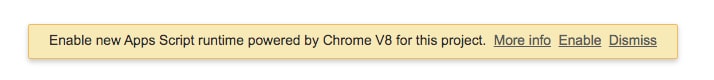
When you open the Apps Script editor, you’ll see a yellow notification bar at the top of your editor window prompting you to enable V8:
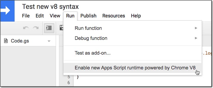
If you don’t see this notification, you can select Run > Enable new Apps Script runtime powered by V8
Save your script to complete the enabling process.
If you need to return to the old version (in the unlikely scenario your script isn’t compatible with the new V8 runtime) then you can switch back to the old Rhino runtime editor.
Select Run > Disable new Apps Script powered by V8.
New Logging In The Apps Script V8 Runtime
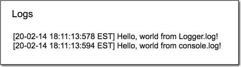
The new V8 runtime logger shows both the Logger.log and console.log results for the most recent execution under the View > Logs menu.
Previously the console results were only accessible via the Stackdriver Logging service.
Here’s an example showing the Logger and console syntax (notice Logger is capitalized and console is not):
function loggerExample() {
  Logger.log("Hello, world from Logger.log!");
  console.log("Hello, world from console.log!")
}
The output in our logger window (accessed via View > Logs) shows both of these results:
Modern JavaScript Features
There are a lot of exciting new features available with modern JavaScript. They look strange at first but don’t panic!
There’s no need to start using them all immediately.
Just keep doing what you’re doing, writing your scripts and when you get a chance, try out one of the new features. See if you can incorporate it in your code and you’ll gradually find ways to use them.
Here are the new V8 features in a vague order of ascending difficulty:
Multi-line comments
We can now create multi-line strings more easily by using a back tick syntax:
// new V8 method
const newString = `This is how we do
multi-line strings now.`;
This is the same syntax as template literals and it greatly simplifies creating multi-line strings.
Previously each string was restricted to a single line. To make multi-line comments we had to use a plus-sign to join them together.
// old method
const oldString = 'This is how we used\n'
+ 'to do multi-line strings.';
Default Parameters
The Apps Script V8 runtime lets us now specify default values for parameters in the function definition.
In this example, the function addNumbers simply logs the value of x + y.
If we don’t tell the function what the values of x and y are, it uses the defaults we’ve set (so x is 1 and y is 2).
function addNumbers(x = 1, y = 2) {
  console.log(x + y);
}
When we run this function, the result in the Logger is 3.
What’s happening is that the function assigns the default values to x and y since we don’t specify values for x and y anywhere else in the function.
let Keyword
The let statement declares a variable that operates locally within a block.
Consider this fragment of code, which uses the let keyword to define x and assign it the variable of 1. Inside the block, denoted by the curly brackets {…}, x is redefined and re-assigned to the value of 2.
let x = 1;

{
  let x = 2;
  console.log(x); // output of 2 in the logs
}

console.log(x); // output of 1 in the logs
The output of this in the logs is the values 2 and 1, because the second console.log is outside the block, so x has the value of 1.
Note, compare this with using the var keyword:
var x = 1;

{
  var x = 2;
  console.log(x); // output of 2 in the logs
}

console.log(x); // output of 2 in the logs
Both log results give the output of 2, because the value of x is reassigned to 2 and this applies outside the block because we’re using the var keyword. (Variables declared with var keyword in non-strict mode do not have block scope.)
const Keyword
The const keyword declares a variable, called a constant, whose value can’t be changed. Constants are block scoped like the let variable example above.
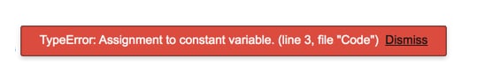
For example, this code:
const x = 1;
x = 2;
console.log(x);
gives an error when we run it because we’re not allowed to reassign the value of a constant once it’s been declared:
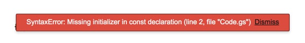
Similarly, we can’t declare a const keyword without also assigning it a value. So this code:
const x;
also gives an error when we try to save our script file:
Spread syntax
Suppose we have the following array of data:
const arr = [[1,2],[3.4],[5,6]];
It’s an array of arrays, so it’s exactly the format of the data we get from our Sheets when we use the getRange().getValues() method.
Sometimes we want to flatten arrays, so we can loop over all the elements. Well, in V8, we can use the spread operator (three dots … ), like so:
const flatArr = [].concat(...arr);
This results in a new array: [1,2,3,4,5,6]
Template Literals
Template literals are a way to embed expressions into strings to create more complex statements.
One example of template literals is to embed expressions within normal strings like this:
let firstName = 'Ben';
let lastName = 'Collins';
console.log(`Full name is ${firstName} ${lastName}`);
The logs show “Full name is Ben Collins”
In this case, we embed a placeholder between the back ticks, denoted by the dollar sign with curly brackets ${ some_variable }, which gets passed to the function for evaluation.
The multi-line strings described above are another example of template literals.
Arrow Functions
Arrow functions provide a compact way of writing functions.
Arrow Function Example 1
Here’s a very simple example:
const double = x => x * 2;
This expression creates a function called double, which takes an input x and returns x multiplied by 2.
This is functionally equivalent to the long-hand function:
function double(x) {
  return x * 2;
}
If we call either of these examples and pass in the value 10, we’ll get the answer 20 back.
Arrow Function Example 2
In the same vein, here’s another arrow function, this time a little more advanced.
Firstly, define an array of numbers from 1 to 10:
const arr = [1,2,3,4,5,6,7,8,9.10];
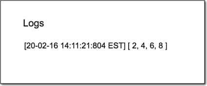
This arrow function will create a new array, called evenArr, consisting of only the even numbers.
The filter only returns values that pass the conditional test: (el % 2 === 0) which translates as remainder is 0 when dividing by 2 i.e. the even numbers.
The output in the logs is [2,4,6,8]:
Other Advanced Features
There are more advanced features in V8 that are not covered in this post, including:
Destructuring assignment that allows us to unpack values from arrays or objects, into distinct variables.
Classes, which are a means to organize code with inheritance. Think of this as creating a blueprint from which copies can be made.
I’m still exploring them and will create resources for them in the future.
Migrating Scripts To Apps Script V8 Runtime
The majority of scripts should run in the new V8 runtime environment without any problems. In all likelihood, the only adjustment you’ll make is to enable the new V8 runtime in the first place.
However, there are some incompatibilities that may cause your script to fail or behave differently.
But for beginner to intermediate Apps Scripters, writing relatively simple scripts to automate workflows in G Suite, it’s unlikely that you’ll have any problems.