Formula Challenge #4: Sort A Column By Last Name

This Formula Challenge originally appeared as Tip #108 of my weekly Google Sheets Tips newsletter, on 29 June 2020. Sign up so you don’t miss future Formula Challenges!

Sign up here so you don’t miss out on future Formula Challenges:

 

Find all the Formula Challenges archived here.

The Challenge: Sort A Column By Last Name

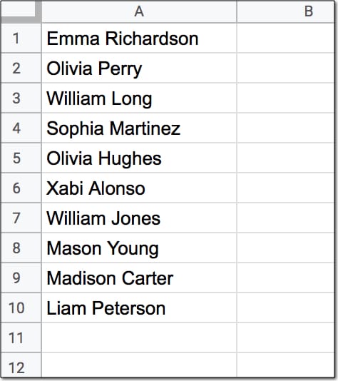
Start with a list of any ten two-word names in column A, like so:

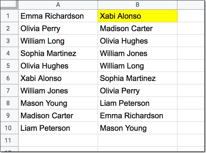
Your challenge is to create a single formula in cell B1 (shown in yellow below) that sorts this list alphabetically by the last name, like this:

Assumptions:

• The names to sort are in the range A1:A10
• Each name consists of a first name and last name only, with a single space between them
• None of the names have prefixes or suffixes
• The formula in cell B1 should output the full names in range B1:B10

Solutions To Sort A Column By Last Name

I received over 90 replies to this formula challenge with at least 10 different methods for solving it. This was super interesting to see!

Congratulations to everyone who took part.

I learnt so much from the different replies, many of which proffered shorter and more elegant solutions than my own original formula.

Here I present the best 4 solutions, chosen for their simplicity and elegance.

There’s a lot to learn by looking through them.

---

1. SORT/INDEX/SPLIT method

Solution:

Use this formula in cell B1 to sort the data alphabetically by the last name:

This is a beautiful solution.

It’s deceptively simple, as you’ll see below when we break it down. And yet, only a handful of people submitted this solution.

How does this formula work?

Let’s use the onion method to peel back the layers and build this formula in steps from the innermost layer.

Step 1:

Enter this formula as a starting point:

The SPLIT function takes the range A1:A10 as an input and splits the names on the space character. That works in this example because of our rigid assumptions that all names are two-word names.

The output is a single row with the name split across two cells. (Adding an ArrayFormula would give an output of all ten names, but it’s not required when we plug this split into the INDEX function.)

Step 2:

Wrap the formula from step 1 in an INDEX function:

Leave the row argument (the second argument) in the function blank and choose column 2 in the column argument (the third one). This formula outputs the list of second names, still in the original order, however.

Step 3:

The SORT function takes three arguments: the range to sort, the column to sort on, and whether to sort ascending or descending.

So A1:A10, the range containing the full names, is the range we want to sort.

Then the column of last names created in step 2 is the column we want to sort on. This is our second argument.

Then the third argument is a TRUE or 1 to indicate we want to sort the names ascending.

So plugging these three arguments into the SORT function gives the following formula:

This formula can be modified to include the whole of column A if there are more than 10 names. Simply change the range from A1:A10 to A1:A as follows:

---

2. QUERY method

Solution:

Use this formula in cell B1 to sort the data alphabetically by the last name:

Step 1:

Step 1 is the same as the step 1 in solution 1 above, and uses the SPLIT to separate the names into first and last names in separate columns:

Step 2:

Step 2 combines these two split columns with the original column of names using array literals to construct an array of full name, first name and last name.

The ArrayFormula wrapper is necessary to output all 10 values in this example.

Step 3:

The array created by step 2 is used as the input data range in the QUERY function in step 3:

Since the input range of the QUERY function is constructed with the curly brace notation {…} we are required to use the Col1, Col2, etc. notation to access the columns. The query clause is pretty simple. Select only column 1 of the array (the full name) but sort by column 3 (the last name).

Note, the ArrayFormula can be brought outside the QUERY to be the outer wrapper.

This formula can be extended easily to the whole of column A by changing the range to A1:A and adding a WHERE clause to filter out the blank rows:

---

3. REGEX method I

Solution:

Use this formula in cell B1 to sort the data alphabetically by the last name:

If the first solution was the shortest and simplest, then this is perhaps the most elegant.

It only references the data range A1:A10 once, whereas all the other solutions presented here reference the data range twice.

Step 1:

Use the Google Sheets REGEXEXTRACT function to split the data into three columns of full name, first name and last name:

This formula uses numbered capturing groups to capture the data, denoted by (.*) and ( .*) with the second having a space. The .* simply says match zero or more of any character.

In other words, the (.*)( .*) construction separates into first and last names. Adding another matching group with the additional parentheses ((.*)( .*)) also matches the full name.

These three columns are passed into the SORT function in STEP 2:

Step 2:

The data is sorted on column 3 containing the last name. The 1 represents a TRUE value which sorts the data ascending from A-Z.

Step 3:

In the final step, we use the INDEX function to return only the first column, which has the full name.

---

4. REGEX method II

Solution:

Use this formula in cell B1 to sort the data alphabetically by the last name:

This is the same method as the first solution, but uses REGEXEXTRACT instead of INDEX/SPLIT. So it’s one less function, but the REGEXEXTRACT function is much harder to understand than the INDEX/SPLIT combination for those unfamiliar with the black magic of regular expressions.

Step 1:

Use the REGEXEXTRACT function to extract the last names from the data:

The (?: ) is a non-capturing group matching the space. In other words the REGEXEXTRACT matches the space but doesn’t extract it.

The \w character matches word characters (≡ [0-9A-Za-z_]) and the * means match zero or more word characters but prefer more.

The parentheses ( ) around the \w* make it a captured group so it’s extracted.

See, regular expressions are as clear as mud.

Ok, so what’s happening is that it matches on the space, but doesn’t return it. Then it matches on the word group that follows the space and returns that. Hence we get an output range of last names only.

Step 2:

The final step is to sort range A1:A10 using the last names extracted in step 2, and sort them ascending. This step is identical to the implementation in solution 1.

This formula can be modified to include the whole of column A if there are more than 10 names. Simply change the range from A1:A10 to A1:A as follows:

---

There we go!

Four brilliant solutions to an interesting formula challenge.

Please leave comments if you have anything you wish to add.

And don’t forget to sign up to my Google Sheets Tips newsletter so you don’t miss future formula challenges!