Join The Dots Drawing In Google Sheets

This post was born from my ongoing experimentation/obsession with the SPARKLINE function in Google Sheets.

We’ll see how to create a Join-The-Dots game in Google Sheets using only the built-in formulas, no code.

🔗 Grab your own copy of the template at the bottom of this article. 👇

This Join The Dots game works using four techniques:

1. A transparent scatter plot for the numbered dots
2. Checkboxes acting as buttons
3. MAKEARRAY formula to generate drawing coordinates
4. A SPARKLINE formula to draw the line

It’s created entirely with the native built-in functions of Google Sheets and doesn’t use any code.

It’s similar to the Etch-A-Sheet project I did in 2022 and builds on the work done by Tyler Robertson to set up checkboxes as buttons.

How Does This Join The Dots Game Work?

Step 1: Scatter Plot For The Dots

The first step is to set up the “dots”.

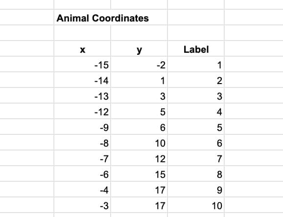
For this, we need a set of 2-D coordinates of the thing you want to draw. For example, a triangle would consist of these coordinate pairs:

(0,0)
(1,2)
(2,0)
(0,0)

where (0,0) represents the bottom left corner of the drawing area.

I also added a third column of sequential numbers, which we show as labels on the chart.

The coordinates for the rabbit picture are available in the template at the end of this post.

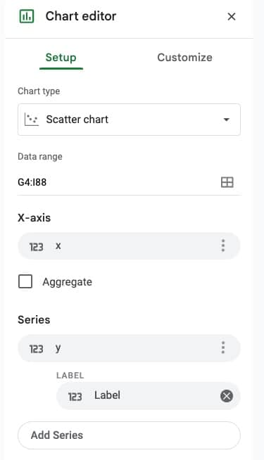
Highlight this data and create a chart: Insert > Chart

Select a Scatter chart with the following settings in the Setup menu:

• X-axis set to the x column in our data
• Series set to the y column in our data
• Add the Label column as a Label to the Series

In the Customize menu, apply the following settings:

• Chart style –> Background color NONE
• Chart style –> Chart border color NONE
• Chart & axis titles –> Remove
• Series –> Set the color to black
• Series –> Add Data labels to the Series, font size 6
• Horizontal axis –> set the font color to white (to hide) and min to -16 and max to 17 (these would change to match the max/min of your drawing coordinates)
• Vertical axis –> set the font color to white (to hide) and min to -18 and max to 18
• Gridlines and ticks –> Remove

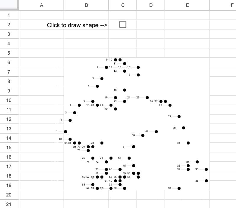
Next we create a larger square canvas by merging cells together (this example uses the range B6 to E19). Overlay the chart on this merged cell.

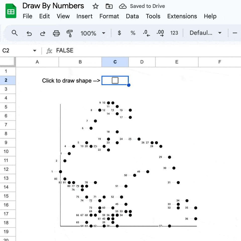
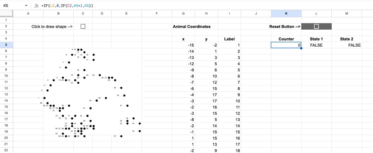
For the animal drawing, it looks like this in our Sheet:

Step 2: Checkbox Control System

Before continuing, I recommend that you read Tyler Robertson’s original article on how this technique works.

Add two checkboxes to your Sheet: one will increment the counter (in cell C2), the other will reset it to 0 (in cell L2).

When a checkbox is toggled, it changes from a TRUE to a FALSE value, or vice-versa.

Knowing that, we use these formulas to setup and increment the counter.

The Counter formula:

State 1 formula:

State 2 formula:

It will look like this in our Sheet:

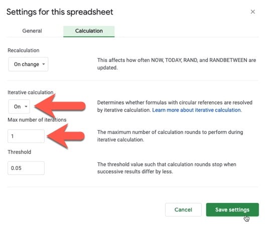
For this to work, the spreadsheet needs to have iterative calculations enabled with the max set to 1 iteration.

Change the settings under the menu File > Settings > Calculation

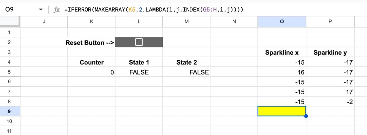
Step 3: Sparkline Coordinates

When the counter checkbox is clicked, the counter grows 1,2,3,4,5,…etc.

This increasing value is fed into a MAKEARRAY function as the number of rows. The number of columns is fixed at 2.

The LAMBDA function inside MAKEARRAY uses the INDEX function to grab the relevant x-y coordinate from the drawing coordinates range.

We wrap the MAKEARRAY formula with an IFERROR function to handle the case when the checkbox has not been clicked yet.

The full formula to generate the data is:

The sparkline needs a set of axes that reach from the min values to the max values to ensure it doesn’t resize with each new set of coordinates.

The following image shows how the Sheet is set up. The main formula is highlighted in yellow, underneath the static coordinates for the sparkline axes.

Step 4: Drawing The Sparkline

Add a simple SPARKLINE formula into the merged cell containing the chart:

(Use the arrow keys to “move into” that cell from an adjacent cell, as the mouse will keep selecting the chart.)

The sparkline coordinates “grow” as the checkbox is clicked and additional coordinates are added to the columns, as shown in this image:

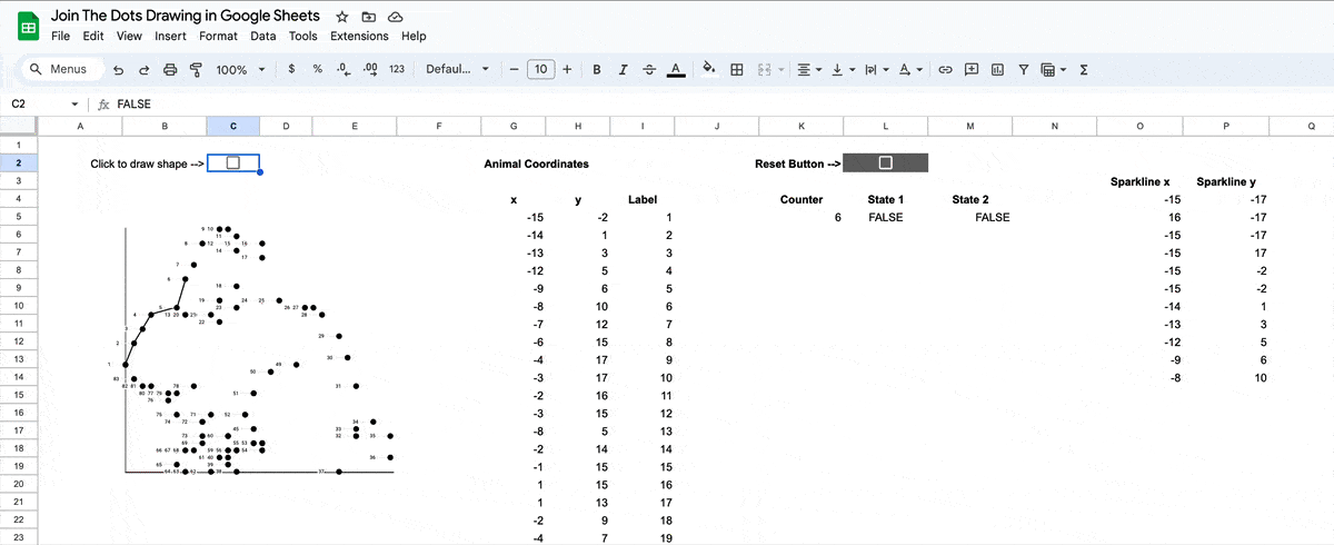
As a consequence, the sparkline itself appears to grow, as the formula recalculates with each change, to give the impression of joining the dots!

Join The Dots Template

🔗 Click here to open a view-only copy >>

Make your own copy: File > Make a copy

(Note: If you are unable to open this file, it’s probably because it’s from an outside organization and my Google Workspace domain is not whitelisted at your organization. Ask your Google Workspace administrator about this. In the meantime, feel free to open it in an incognito window and you should be able to view it.)

If the template does not work, check you have the iterative calculations enabled.

Go to: File > Settings > Calculation

Make sure Iterative Calculations is ON and set to 1 iteration.

If you do make a copy, I’d love to see what you draw with it!

Other Fun Sparkline Projects

For more sparkline fun, check out these other projects:

Google Sheets Formula Clock

Etch A Sheet In Google Sheets

How To Draw The Cantor Set In Google Sheets

Bullet Chart in Google Sheets