Although AI has been around for decades, it’s only really been available to the public in its current form for the past year or so. And with the rise of these generative AI tools, like ChatGPT and Google Bard, AI is more accessible than ever.
But where does AI fit with Google Sheets?
And how do we use AI tools with Google Sheets?
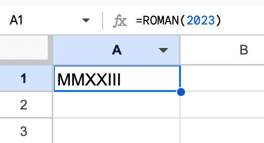
In this post we’re going to look at how to use the most popular AI tools with Google Sheets. You’ll see how easy it is get started and learn that AI isn’t rocket science. It’s simply another useful tool that can save you time when you work with Google Sheets.
Specifically, we’ll look at three ways to use AI tools with Google Sheets:
- Chatbots like ChatGPT or Bard
- Google Sheets Add-Ons
- Via the API and Apps Script (advanced)
Continue reading Three Ways To Use AI Tools With Google Sheets