Recursion in Google Sheets is now possible with the introduction of Named functions, LAMBDA functions, and LET functions. In this post, we’ll explore the concept of recursion and look at how to implement recursion in Google Sheets.
Educator and Google Developer Expert. Helping you navigate the world of spreadsheets & AI.
Recursion in Google Sheets is now possible with the introduction of Named functions, LAMBDA functions, and LET functions. In this post, we’ll explore the concept of recursion and look at how to implement recursion in Google Sheets.
In this post, we’ll build a named function that creates a miniature bullet chart in Google Sheets, as shown in this GIF:
Bullet charts are variations on bar charts that show a primary measure compared to some target value. They’re highly effective because they capture a lot of information in a small, neat design.
To begin with — a warm-up if you like — let’s create a simple version of a bullet chart using a standard sparkline. (This formula featured as Tip 237 in my weekly Google Sheets newsletter. Sign up to get a weekly actionable Google Sheets tip!)
⚡ A template is available at the end of this post.
Continue reading Bullet Chart in Google Sheets with Sparklines and Named Functions
This Formula Challenge originally appeared as Tip #243 of my weekly Google Sheets Tips newsletter, on 27 February 2023.
Congratulations to everyone who took part and submitted a solution!
Sign up for my newsletter to receive future Formula Challenges:
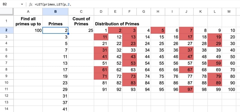
Can you create a single formula that creates the output shown in this image:
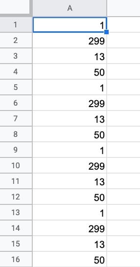
Assume a height of 100 rows.
There were a lot of great solutions! Here are 8 of the best:
=FLATTEN(SPLIT(REPT("1,299,13,50,",25),","))This formula starts with a text representation of the number sequence “1,299,13,50,”.
It uses REPT to repeat the sequence, SPLIT to separate by the commas, and finally FLATTEN (or TRANSPOSE) to convert to a column format.
This is the shortest formula by character count.
=ArrayFormula(FLATTEN(IF(SEQUENCE(25),{1,299,13,50})))In this formula, SEQUENCE generates a column of 25 numbers. An IF formula wrapper then takes each number as an input and, since numbers are truthy values, the IF outputs the array.
The FLATTEN function then stacks into a single column.
=MAKEARRAY(100,1,LAMBDA(i,_,CHOOSE(MOD(i-1,4)+1,1,299,13,50)))The MAKEARRAY function generates an array of 100 rows in 1 column. The LAMBDA function uses MOD to create a sequence 1,2,3,4,1,2,3,4,1,2,3,4…
The CHOOSE function converts the 1,2,3,4 into the sequence 1,299,13, or 50.
Also, note the use of the underscore “_” to denote the argument in the LAMBDA that is not used in the formula.
=ArrayFormula(CHOOSE(MOD(SEQUENCE(100)-1,4)+1,1,299,13,50))The SEQUENCE function generates a list from 1 to 100. MOD converts this to a repeating sequence 1,2,3,4,1,2,3,4,1,2,3,4,…
The CHOOSE function then sets the final values and the whole is wrapped with ArrayFormula to output the full array.
=ArrayFormula(FLATTEN(SEQUENCE(25,1,1,0)*{1,299,13,50}))The SEQUENCE function generates 25 rows of 1’s, which is multiplied by the array literal {1,299,13,50}. This creates 4 columns, one for each number in the sequence. FLATTEN then stacks them in a single column.
=ArrayFormula(FLATTEN( MMULT(SEQUENCE(25,1,1,0),{1,299,13,50})))This is essentially the same as the previous solution (#5) but uses the MMULT function to multiply the two arrays.
=ArrayFormula(1*FLATTEN({1,299,13,50}&LEFT(F1:F25,0)))This unusual solution uses the LEFT function to create an empty array of 25 rows, because the length is set to 0.. It can use any column except the one containing the formula itself.
=ArrayFormula(

SWITCH(MOD(ROW(A1:A100),4),

1,ROW(),

2,ROW()+298,

3,ROW()+12,

ROW()+49))
This novel approach uses MOD with the ROW function to generate a repeating sequence. This is fed into a SWITCH function to convert to the desired output.
The newly released TOCOL function could also be used in this challenge, but was unavailable at the time of writing.
The best way to explore and understand these formulas is to use the Onion Framework to create them for yourself, starting with the innermost function.
Coming hot on the heels of last year’s batch of new lambda functions, Google recently announced another group of new analytical functions for Sheets.
Included in this new batch are the long-awaited LET function, 8 new array manipulation functions, a new statistical function, and a new datetime function.
Let’s begin with a look at the new array functions. The LET function is at the end of the post.
Continue reading 11 New Analytical Functions In Google Sheets For 2023
 💡 Learn more
The XMATCH function in Google Sheets is a new lookup function in Google Sheets that finds the relative position of a search term within an array or range. It’s an evolution of the original MATCH function.
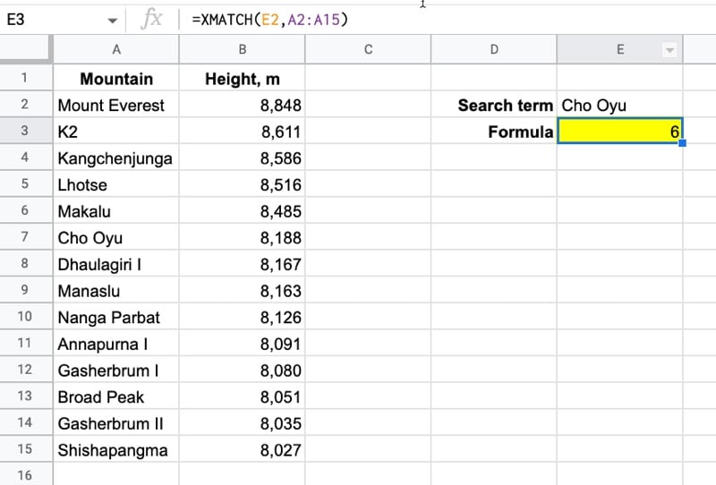
Here’s a simple XMATCH function that finds the position of the search term “Cho Oyu” in the list of the highest mountains in the world:
=XMATCH(E2,A2:A15)In the Sheet:
And here’s how it works:
It looks for the search term from cell E2 (“Cho Oyu”) in the range A2:A15, then returns the position of the search text within this range. Note that the result is relative to the range, irrespective of the row number.
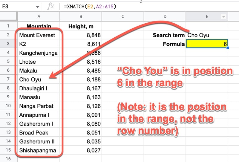
Notice how, unlike a regular MATCH function, you don’t have to specify the “0” search type for an exact match. It chooses the exact match, which is by far the most common use case, by default (in contrast to the MATCH function where you have to add the 0 to explicitly confirm exact matching). More on the search types below.
🔗 Get this example and others in the template at the bottom of this article.