A Guide To Named Functions In Google Sheets

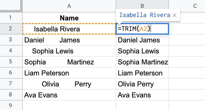
Named Functions in Google Sheets let you save and name your own custom formulas and then re-use them in other Google Sheet files.

Wow! How exciting is that?!? (Hint: VERY)

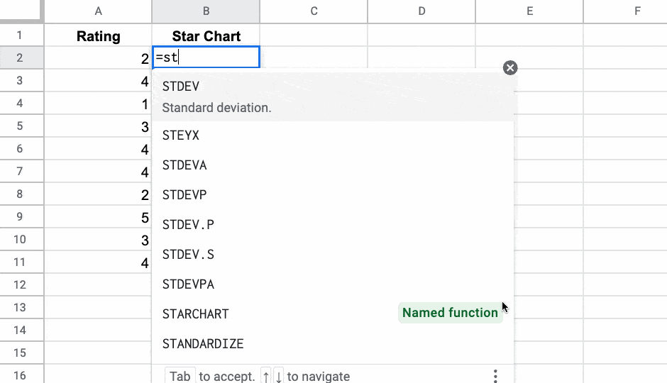
For example, here I’m using a named function I created called STARCHART to add a rating chart to my Sheet:

Named Functions in Google Sheets Star Chart Example

And here I’m using a named function I called UNPIVOT to turn my wide data into a tall format:
Continue reading A Guide To Named Functions In Google Sheets

How To Use The TRIM Function In Google Sheets To Clean Your Data

The TRIM function in Google Sheets removes unwanted spaces around text.

Trim Function Example In Google Sheets

TRIM removes the leading, trailing, and repeated spaces in the text values in column A.

The formula is:

=TRIM(A2)

πŸ”— Get this example and others in the template at the bottom of this article.

Continue reading How To Use The TRIM Function In Google Sheets To Clean Your Data

How To Use The Choose Function In Google Sheets

The CHOOSE Function in Google Sheets lets you choose between different options.

It’s a lookup function, akin to a limited VLOOKUP rather than an alternative to the IF function.

It takes an index number and returns a value at that numbered position from the list of possible options.

Here’s a simple example:

=CHOOSE(1,"A","B")

which will output:

CHOOSE Function in Google Sheets

The first argument is the index number: 1.

Subsequent arguments are possible choices. The CHOOSE function returns the value at index position 1 in this case, i.e. “A”.

If I changed the index number to 2, the CHOOSE function would output “B”.

πŸ”— Get this example and others in the template at the bottom of this article.

Continue reading How To Use The Choose Function In Google Sheets

How To Create Arrays In Google Sheets (a.k.a. Array Literals)

Arrays in Google Sheets are collections of data, consisting of rows and columns. You can use arrays in formulas in the same way that you use regular A1-type ranges.

You construct arrays in Google Sheets with curly brackets: { }

They’re also known as ARRAY LITERALS.

Continue reading How To Create Arrays In Google Sheets (a.k.a. Array Literals)

How To Rank Data In Google Sheets With The RANK Function

Google Sheets has three functions to rank data: the RANK function, the RANK.EQ function, and the RANK.AVG function.

All three functions return the rank (position) of a value in a dataset.

RANK and RANK.EQ are equivalent to each other and return the top rank for values that are tied. RANK.EQ is the more modern notation, to explicitly differentiate itself from RANK.AVG.

The RANK.AVG function differs by returning the average rank of any entries that are tied.

Consider this dataset showing the three RANK functions in action, with a tie highlighted in yellow:

All Rank Functions

Both RANK and RANK.EQ display the tied values with the rank 5, whereas RANK.AVG shows the average rank of 5.5 (i.e. the average of position 5 and position 6).

The RANK formula in column C:

=RANK(B2,$B$2:$B$11)

And RANK.EQ formula in column D, giving the same answer:

=RANK.EQ(B2,$B$2:$B$11)

Finally, RANK.AVG formula is in column E:

=RANK.AVG(B2,$B$2:$B$11)

πŸ”— Get this example and others in the template at the bottom of this article.

Continue reading How To Rank Data In Google Sheets With The RANK Function