formulas Archives - Page 8 of 14 -

How To Use The IMPORTRANGE Function In Google Sheets To Transfer Data From One Sheet To Another

Since Google Sheets are files in the cloud, not on your desktop, you can’t click on a cell in a different Sheets file to connect them.

Instead, you use the IMPORTRANGE function in Google Sheets to connect Google Sheet files and import data from one Sheet file into another.

Once set up, the function will automatically sync with the source data so that changes are reflected in the destination Sheet.

IMPORTRANGE In Google Sheets

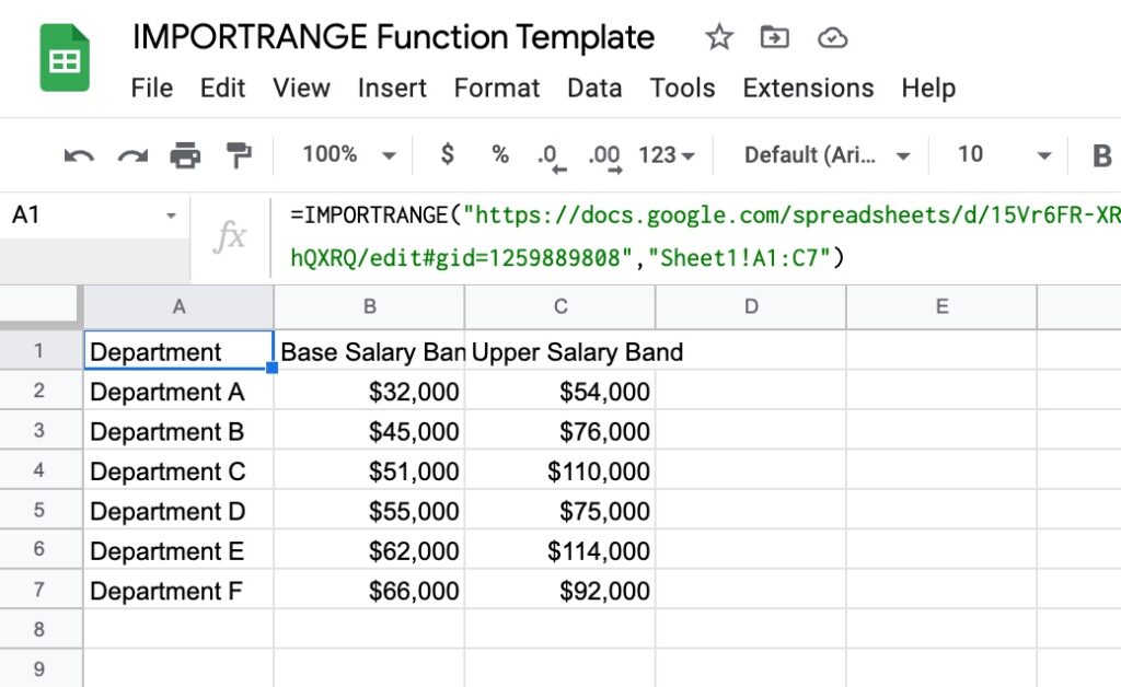
If you look closely, you’ll see a URL in the formula — the URL of the source Google Sheet file, where the data is being imported from.

Continue reading How To Use The IMPORTRANGE Function In Google Sheets To Transfer Data From One Sheet To Another

How To Highlight The Top 5 Values In Google Sheets With Formulas

In this post, you’ll learn how to find and highlight the top 5 values in Google Sheets.

For all the examples that follow, we’ll use this dataset, which is available in the downloadable template at the end of this post:

Example Dataset

We’ll see how to highlight the rows with the top 5 values, as well as how to extract those values using SORTN.

Continue reading How To Highlight The Top 5 Values In Google Sheets With Formulas

How To Mimic Radio Buttons With Formulas and Checkboxes

In this post, we’ll look at how to mimic radio buttons with formulas and checkboxes in Google Sheets.

Radio button behavior with checkboxes and formulas

This formula method has one limitation: you have to uncheck the current selection before you can check a different one.

With true radio buttons, when you click any button it will unselect the other one for you. You don’t have to do the extra step of manually unselecting it first.

For that reason, I recommend using an Apps Script method to create true radio buttons in Google Sheets.

However, the formula method presented in this post is useful if you don’t have access to Apps Script or simply don’t want to add code to your project.

Continue reading How To Mimic Radio Buttons With Formulas and Checkboxes