Tag: Google Sheets

The Google Sheets SUMIFS function is used to sum ranges based on conditional tests. In other words, the SUMIFS in Google Sheets adds values to a total only when multiple conditions are met.

Suppose we want to calculate the total for Large products in New York:

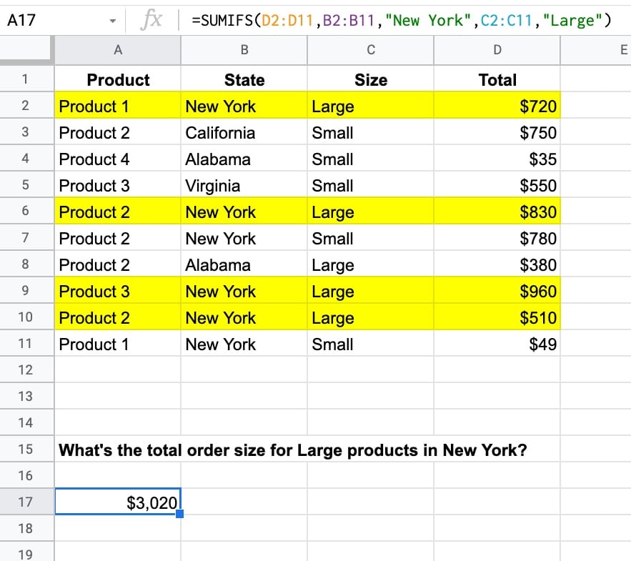
The SUMIFS function to calculate the total for two conditions, Large and New York, is:

which gives an answer of $3,020.

In this case, there are four rows, highlighted in yellow, that match the criteria of New York in column B and Large in column C.

The total values of these four rows are added together by the SUMIFS function, all the other rows are discarded.

🔗 Get this example and others in the template at the bottom of this article.

Continue reading Google Sheets SUMIFS Function

The SUMIF function in Google Sheets is used to sum across a range of cells based on a conditional test. The SUMIF function only adds values to the total when the condition is met.

Let’s see an example. Suppose we want to calculate the total order value for John only:

The SUMIF formula that calculates the total order value for John is:

which gives an answer of $2,059.

The formula tests column A for the value “John”, and, if it matches John, adds the value from column C to the total. I’ve highlighted the four rows in yellow that are included.

🔗 Get this example and others in the template at the bottom of this article.

Continue reading How To Use Google Sheets SUMIF Function

The VLOOKUP function in Google Sheets is a vertical lookup function. You use it to search for an item in a column and return data from that row if a match is found.

In the following example, we use a VLOOKUP formula to search for “Charles Dickens” in column 1. When we find it, the formula returns the value from the 4th column of the lookup table to give a result of $299.

In this example, the VLOOKUP function is:

Let’s break this formula down:

B8 is the search term: “Charles Dickens”

The VLOOKUP looks down the first column of the lookup table: A2:D5

If it finds the search term, it then looks across that row to the column indicated by the Index number: 4

It then returns the value from column 4 as the answer, which is $299 in this example.

The final argument is false, meaning this is an exact match.

VLOOKUP can also handle approximate matching as well as wildcard searches. These more advanced use cases are explored further below.

Continue reading VLOOKUP Function in Google Sheets: The Essential Guide

The Google Sheets COUNTIFS function is used to count items in ranges with multiple test criteria.

It works like a COUNTIF function, but lets you include more than one conditional test.

Here’s an example with a small real estate example dataset:

How can we count the number of deals for apartments and buyers?

To count them, we use a COUNTIFS function:

There are three rows that are apartments AND buyers, highlighted in yellow.

Continue reading Google Sheets COUNTIFS Function