 💡 Learn more
Learn more about working with Lambda Functions, Named Functions, and X-Functions in the FREE Lambda Functions 10-Day Challenge course
The XMATCH function in Google Sheets is a new lookup function in Google Sheets that finds the relative position of a search term within an array or range. It’s an evolution of the original MATCH function.
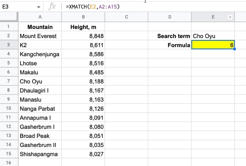
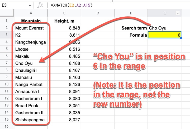
Here’s a simple XMATCH function that finds the position of the search term “Cho Oyu” in the list of the highest mountains in the world:
=XMATCH(E2,A2:A15)In the Sheet:
And here’s how it works:
It looks for the search term from cell E2 (“Cho Oyu”) in the range A2:A15, then returns the position of the search text within this range. Note that the result is relative to the range, irrespective of the row number.
Notice how, unlike a regular MATCH function, you don’t have to specify the “0” search type for an exact match. It chooses the exact match, which is by far the most common use case, by default (in contrast to the MATCH function where you have to add the 0 to explicitly confirm exact matching). More on the search types below.
🔗 Get this example and others in the template at the bottom of this article.