Google announced Named Functions and 9 other new functions on 24th August 2022.
The biggest news here is the new feature called Named Functions. Named Functions let you save and name your own custom formulas, built with regular Sheets functions, and then re-use them in other Google Sheet files. It’s a HUGE step toward making formulas reusable.
Let’s look at the named functions and the 9 new functions:
- Named Functions
- LAMBDA Function
- MAP Function
- REDUCE Function
- MAKEARRAY Function
- SCAN Function
- BYROW Function
- BYCOL Function
- XLOOKUP Function
- XMATCH Function
 💡 Learn more
Learn more about working with Lambda Functions, Named Functions, and X-Functions in the FREE Lambda Functions 10-Day Challenge course
1. Named Functions
Named Functions in Google Sheets let you save and name your own custom formulas, using all the built-in functions.
That complex financial formula you created… sure, turn it into a named function called =BENFINANCE(input1,input2,…) and use that instead!
And best of all, you can re-use these named functions in other Google Sheet files.
Here’s an example of a named function I created, called STARCHART, that draws mini star rating charts and can be reused in other Sheets:
Learn more about Named Functions
2. LAMBDA Function
The LAMBDA function in Google Sheets creates a custom function with placeholder inputs, instead of the usual A1 type cell or range references.
The main use case for the LAMBDA function is to work with other new lambda helper functions, like MAP, REDUCE, SCAN, MAKEARRAY, BYCOL, and BYROW.
LAMBDA functions are also the underlying technology for Named Functions, which we saw above.
Here’s an example LAMBDA function to calculate percent change:
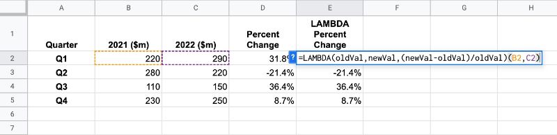
In this case though, you’d be better off creating a named function called PERCENTCHANGE rather than creating this lambda function explicitly.
Learn more about the LAMBDA function
3. MAP Function
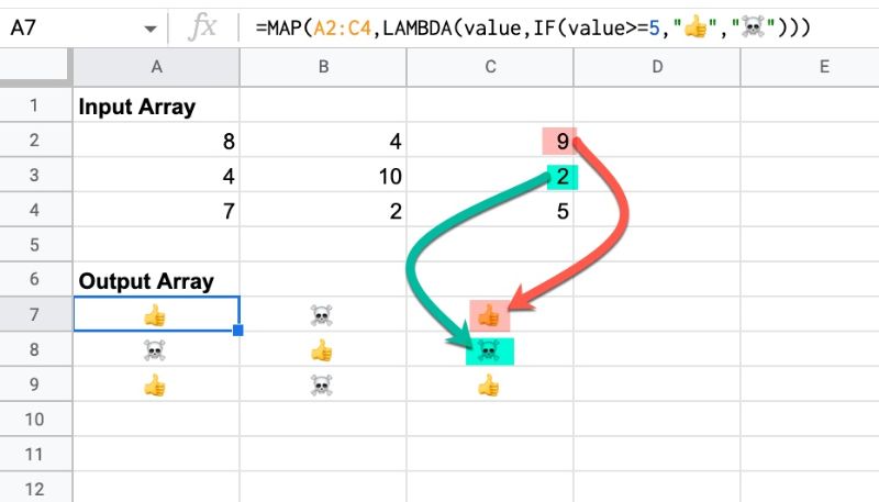
The MAP function in Google Sheets creates an array of data from an input range, where each value is “mapped” to a new value based on a custom LAMBDA function.
It’s the same idea as the MAP function in programming, a way to loop over an array of data and do something with each element of the array.
I think this formula is going to be super useful!
Here’s how the MAP function works, showing a silly transformation of values into emojis using an IF function as the lambda expression:
Learn more about the MAP Function
4. REDUCE Function
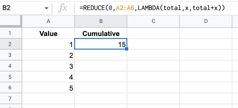
The REDUCE function in Google Sheets operates on an array (like the MAP function). It turns that array input into a single accumulated value, by applying a custom LAMBDA function to each element of the array. I.e. it reduces an array down to a single value.
For example, this simple REDUCE function calculates a cumulative total (yes, using the SUM function is easier, but this reduce example is just for illustration):
Learn more about the REDUCE Function
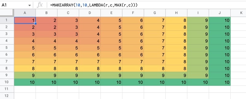
5. MAKEARRAY Function
The MAKEARRAY function in Google Sheets generates an array of a specified size, with each value calculated by a custom lambda function.
It’s like the SEQUENCE or RANDARRAY functions, except that in this case a lambda function is applied to each value in the array, so you can generate more complex arrays.
The lamba function has access to the row and column indices for each value.
Here the lambda evaluates the max of the row and column indices and then I added a heat map to that.
Learn more about the MAKEARRAY function
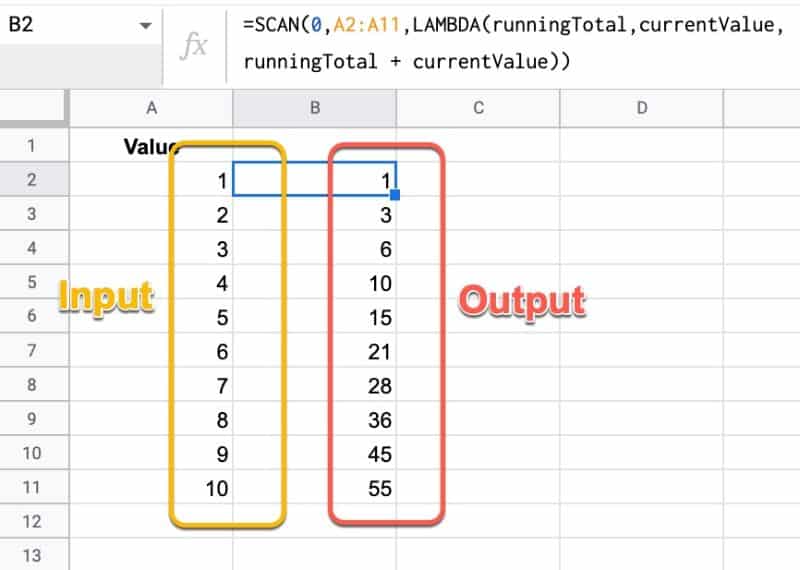
6. SCAN Function
The SCAN function in Google Sheets scans an array by applying a LAMBDA function to each value, moving row by row. The output is an array of intermediate values obtained at each step.
The most obvious application to create running totals of your data, like so:
Learn more about the SCAN Function
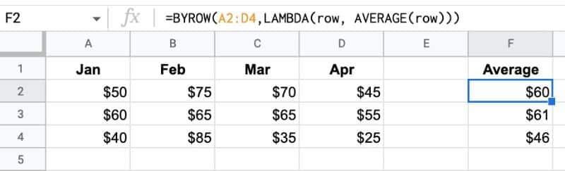
7. BYROW Function
The BYROW function in Google Sheets operates on an array or range and returns a new column array, created by grouping each row to a single value.
The value for each row is obtained by applying a lambda function on that row.
For example, we can use a single BYROW formula to calculate the average score of all three rows in the input array:
Learn more about the BYROW function
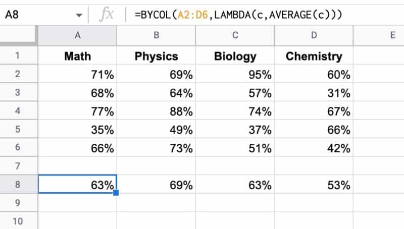
8. BYCOL Function
The BYCOL function operates in the same way as the BYROW function, but groups each column to a single value and returns a new row array.
In this example, the BYCOL formula outputs a row of average values:
Learn more about the BYCOL function
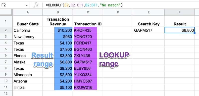
9. XLOOKUP Function
Yes! We have the awesome XLOOKUP function in Google Sheets now!!
It’s a more powerful and flexible version of the VLOOKUP function. It shares some similar capabilities to the INDEX/MATCH combination formulas.
XLOOKUP can lookup to the left, from the bottom up, and even use binary search if you’re working with really large datasets.
Here’s an example of the XLOOKUP performing a leftward lookup:
Learn more about the XLOOKUP Function
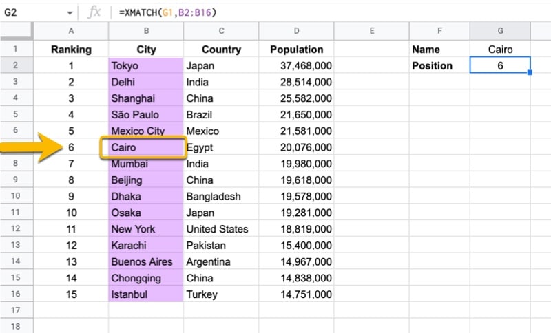
10. XMATCH Function
Last but not least is the XMATCH function, a more powerful and flexible version of the MATCH function.
It has more matching modes and search options than the plain MATCH function.
Here’s a simple XMATCH example:
Extraordinary! I loved it! Thanks for explaining these new functions I was really waiting for for so long!
Enjoy them!
I’m LOVIN IT!
This is beyond awesome! Thank you for alerting us.
I know, right!?! Can’t wait to see what everyone builds with them.
Sir I follows all your posted formulas
I have a question please suggest- For XMATCH , if we have duplicates vales as reference for the same and then what will happen?
I’ll publish a dedicated blog post for the XMATCH function soon!
Thanks Ben. I really enjoy your tips and blog posts.
You’re welcome! Cheers.
Really nice, thanks for Info! These Combinations with Lambda are nice.
Yes, I think map and reduce will prove to be hugely useful functions.
Wow, these blur the lines between functions and Scripting! I think they may prove the gateway drug to Scripting for many people. HUGE game changer. Read it here first and happy to Share to the news!
Yes, it’s really exciting. I’m particularly happy about the reusability aspect.
As you say, the lines are blurring! Once you start writing lambda functions in Sheets, you’re basically already coding 😉
Yes! This is exactly where I’ll be going with this. We’ve basically got a database growing from multiple interconnected sheets & scripts, which is only growing in complexity.
Looks like these functions will help “simplify” this in many ways, which we desperately need for long term sustainability.
Cannot wait to start playing around!
So cool!! Is it possible to force XLOOKUP() to be exact match and not closest match?
Yes. See https://www.benlcollins.com/spreadsheets/xlookup-function/
Thanks, Brian!
Wow! What an update and what an email to wake up to. This takes things to the next level, I’m really looking forward to these new tutorials Ben, thanks for informing 🙂
You’re welcome! Enjoy the new functions.
Wow !
finally, we have what excel has. Finally sheets have lambda…looking forward to coding ….
Thanks a lot my man for sharing the updates.
I am so thankful to you
Great news! I wish they’d added LET too, but named functions are enough to make my day 😉
Do you know if REFERENCE and SINGLE are now official?
Yes, LET would have been useful, but my guess is they decided named functions was enough.
Have not heard anything about REFERENCE and SINGLE!
On the face of it the omission of LET is puzzling, given the general trend of Google Sheets to mimic as many of Excel’s functions as possible. However I suspect that the answer here lies with the fact that a plain ‘anonymous’ LAMBDA (i.e. written in a cell and not as a named function) is functionally equivalent to a LET, albeit with different syntax. I wonder if Google Sheets will convert any LETs in imported Excel files automatically on this basis?
I see LET defined now: https://support.google.com/docs/answer/13190535?hl=en&ref_topic=1240289#
But it’s still showing as an undefined function.
As always, excellent tips, news and help .
Thank you very much, Ben
You’re welcome!
In the google sheets I can not see new functions like map, reduce and lamda. Do I need to do something to enable them?
No, they will show up within the next 2 weeks during the gradual rollout.
Thank you very much for your valuable help. We are following you all the time.
You’re welcome!
Thank you Ben,
This has been super helpful and the XLookup function is just fantastic.
Lambda needs a bit of exploring but it’s great to have it!
Hi Piotr, you’re welcome. Yes, these new functions are a great step forward.
Many of these examples (maybe because they are rudimentary) I would currently use ARRAYFORMULA for. Maybe a difference is that ARRAYFORMULA doesn’t accept functions that are geared towards operations on a range (SUM, COUNT, MAX, etc) and it seems like LAMBDA and it siblings will.
It would be helpful if you could outline possible other differences.
Yes, these examples are fairly simple by design, to help understand the functional concept.
For sure, there is some overlap between what an array formula and these new lambda functions do, but we’ll see differences emerge as people use them. If you are familiar with programming, then writing these lambda-style functions is more logical and arguably easier than array formulas.
I just discovered COUNTUNIQUEIFS – or am I late to the party?
Nice find! It’s not in the documentation (yet). Do you have a good use case for it?
FYI, the initial announcement has been updated by Google and the rollout start date pushed to September 6th, meaning that the features could come as late as September 21st for some accounts.
I have 2 accounts that got the ability to use lambdas and named functions – albeit without functional helpers such as map / reduce that can be emulated anyway with arrayformulas, and a 3rd account that has no support yet for these new functions (unfortunately it is the workspace of my main customer,).
Thanks for the update, JR! I think they’re trying to speed up the rollout now, so hopefully, folks won’t have to wait as long as Sep 21st.
Hey guys, anyone else still waiting? Got the update to my private account, but not to my workspace business basic yet 🙁
Hi Ben, a specific question for you: do you know any ways of using these new lambdas & helper functions to replicate a SUMIFS that spills as an array? It seems like something that should be possible, but I haven’t been able to figure anything out yet. To me, this is a “holy grail” hope for the lambdas, to be able to “fix” the big gap Sheets has with the various aggregation functions that can’t be made to work with ArrayFormula. SUMIFS is the top of my array wish list for sure.
Woah, I spent some time reading & testing and the answer is yes, MAKEARRAY can be used to turn (probably) any SUMIFS, COUNTIFS, SUM, etc. into an array formula.
The trick is to turn any single row reference into an INDEX() and use the MAKEARRAY to run the function row by row.
It’s a bit tough to explain in a comment box, but if your function was SUMIFS( $C$4:$C$10, $A$4:$A$10, A4), ie sum values in column C where the value in column A matches the row’s value. Then the lambda array version would be:
MAKEARRAY( ROWS($A$4:$A$10),1, LAMBDA(r,c, SUMIFS( $C$4:$C$10, $A$4:$A$10, INDEX($A$4:$A$10,r,c)) ))
The final A4 reference has become an INDEX for the row and column of the MAKEARRAY to run through, which is passed to the LAMBDA as r & c.
Sorry, that’s super complex, but it does work, and here’s where it gets good: you can turn that whole MAKEARRAY LAMBDA bit into a Named Function so you just have to feed it a range and all the complex bits inside just work. This is game-changing for sure.
Ben, I would love to see a blog post about this method in your characteristic clarity. I can’t do it justice here. 🙂
For a real game-changer, turn this into a Named Range and you can now run GOOGLEFINANCE calls with a single array formula:
=MAKEARRAY(ROWS(range),1, LAMBDA(r,c, GOOGLEFINANCE( INDEX(range,r,c), “price”) ))
Can you elaborate on this? I can’t get your formula to work
Hello Ben!
I tried using the XMATCH function but it says “Unknown function”. What does one need to do in order to be able to use the function?
I get that on all of these functions, but if I reload the page it works. Not ideal, but I can test the functionality until they load the functions properly into the app.
Is it not possible to use IMPORTRANGE with XLOOKUP like you can with VLOOKUP to get data from another google sheet?
Named Functions work for me but break when I refresh the page whereafter all the cells with NFs show “Error: Loading data…” forever. I wonder if it’s because I also have Apps Script code and there’s a conflict, i.e. if parts of the GAS code don’t interpret right. Does anyone here know “where” the NF code lives and whether there may be conflicts with sheet-bound apps scripts?
Doing your free 10 Day Challenge course on this one, Is there a way to do SUMIFS inside of an array or by using lambda with helpers?
SUMIF works fine with helper BYROW, and I guess SUMIFS would work fine too
Wow. After 50 years of spreadsheets, there’s *FINALLY* an elegant solution for creating RUNNING TOTALS!!!
Thanks for using that as your example , Ben.
P.S. My first use was to create 2 cells below a list of transfer transactions (i.e. pairs of transactions between banks, each one with a corresponding mate with an amount opposite of the other).
10.00 Credit Card A
-10.00 Bank X
30.00 Credit Card B
-30.00 Bank X
40.00 Credit Card B
-40.00 Bank Y
=sum(A1:A6) # 0.00
=reduce(0, A1:A6, lambda(flow, amount, flow = flow + abs(amount)/2) # 80.00
The sum was $0.00, as it should be, and I used conditional formatting to make it green, indicating that everything balanced.
But a net of $0.00 doesn’t really give an idea of how much flowed backforth, so I figured each side contributes 1/2 to to the financial flux, and added it up! In this case, $80 flowed through the “pipe”.
Nice!!!!
ONE EXAMPLE OF NAMED FUNCTION WRITTEN BY ME
=ARRAYFORMULA(LET(KKKK,SORT(FY_SERIES_NO_OF_FY(QWk!$L$3,12),1,0),IFERROR(CHOOSE(
FILTER(SEQUENCE(COUNTA(QWk!$J$4:$J)),FILT_OUT_BLNKS(QWk!$J$4:$J)=QWk!$L$2),
IF(SELECTOR=”W”,
LET(KK,SORT(MONTH_SERIES_SIMPLE(QWk!$H$4,12),1,0),LL,MAP(KK,LAMBDA(MTH, ARRAYFORMULA(LET(K,EXP_SET_MTH(MTH),P,DAY(CKL(K,1)),TOROW(MAP(SEQUENCE(5,1,1,7),SEQUENCE(5,1,7,7),LAMBDA(F,T,IFERROR(SUM(FILTER(IF(ISERROR(MATCH(CKL(K,2),IF(QWk!$E$3=””,0, STEX(FILTER(ExceptLU!$C$1:$C$4,ExceptLU!$A$1:$A$4=QWk!$E$3),0,2)),0)),CKL(K,3),0),P>=F,P=2))))}),
NEEDS_FYS(KKKK,Needs_Lux!$A$2:$L))),
SEG_GROUPING(),
STR_TO_QTR(KKKK,201001,DIG_CNV(StuP!$B$3,5,10)),
STR_TO_QTR(KKKK,201401,DIG_CNV(StuP!$B$4,5,10)),
LET(L,KKKK,K,MAP(L,LAMBDA(FY, MAP(TRANSPOSE(QWk!$S$13:$S$17),LAMBDA(ITEM, LET(X,EXP_SET_FY(FY),IFERROR(SUM(FILTER(CKL(X,3),CKL(X,4)=SE_CODE(ITEM))))))))),{L,K,SUM_ROWS(K)})
))))