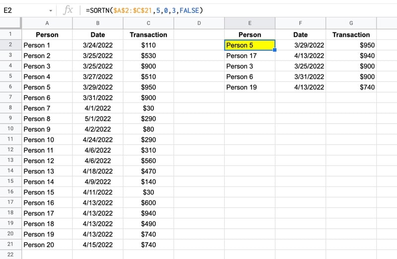
The LARGE function in Google Sheets returns the n-th largest value from a dataset.
For example, you could use large to determine the 5th largest value in a dataset, the 10th largest, the 50th largest, etc.
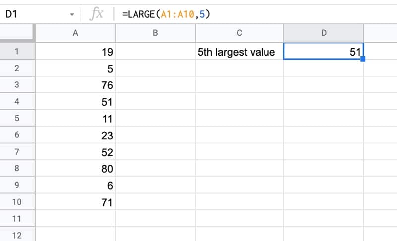
The formula to find the 5th largest value in this example is:
=LARGE(A1:A10,5)🔗 Get this example and others in the template at the bottom of this article.