“If you can’t measure it, you can’t improve it.” – Peter Drucker
Disclosure: Some of the links in this post are affiliate links, meaning I’ll get a small commission (at no extra cost to you) if you signup.
Trying to have conversations about saving, spending and planning for retirement is infinitely more difficult and more stressful without accurate numbers in front of you.
You fall back on anecdotes and feelings because you have nothing else to go on.
Conversations start with phrases like: “it feels like we haven’t spent much on eating out this month” and they don’t get any better from there.
My wife and I have two beautiful boys, aged 2 and 4, and we’re both ambitious with our careers and work full-time. Life is crazy, crazy busy for us right now.
We’ve found it challenging to find time to manage our family finances, so we’ve been in this position of flying blind without a financial tracking plan in place. We’ve had those frustrating conversations, knowing that if we had better insights into our financial habits we could do a much better job at financial planning.
I want to show you how we changed that.
How we created a system in Google Sheets for tracking our spending habits.
It now only takes us about 10 or 15 minutes each week, so we can focus on understanding our financial situation better, and maximize our saving.
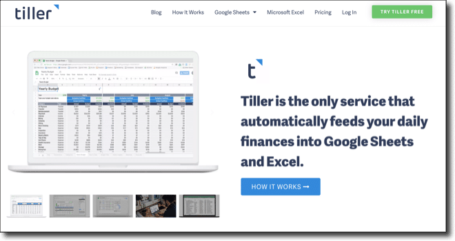
Enter Tiller
Tiller is an amazing tool that connects our bank accounts and credit cards securely to Google Sheets (or Excel), and automatically updates them on a daily basis.
It means we can see all of our financial transactions in one place and do our own custom analysis in Google Sheets.
It’s been transformative for our family’s sanity and helped us get on top of our spending and hit our saving goals.
Tiller has a suite of Google Sheet templates available too, covering spending, saving, budgeting and net worth tracking, so that you can visualize your financial data immediately.
Of course, you can also build your own solutions to answer whatever questions you have.
It costs $79/year, which is tremendous value since you’re getting a fully customizable, automated personal finance tool.
How to setup Tiller with Google Sheets
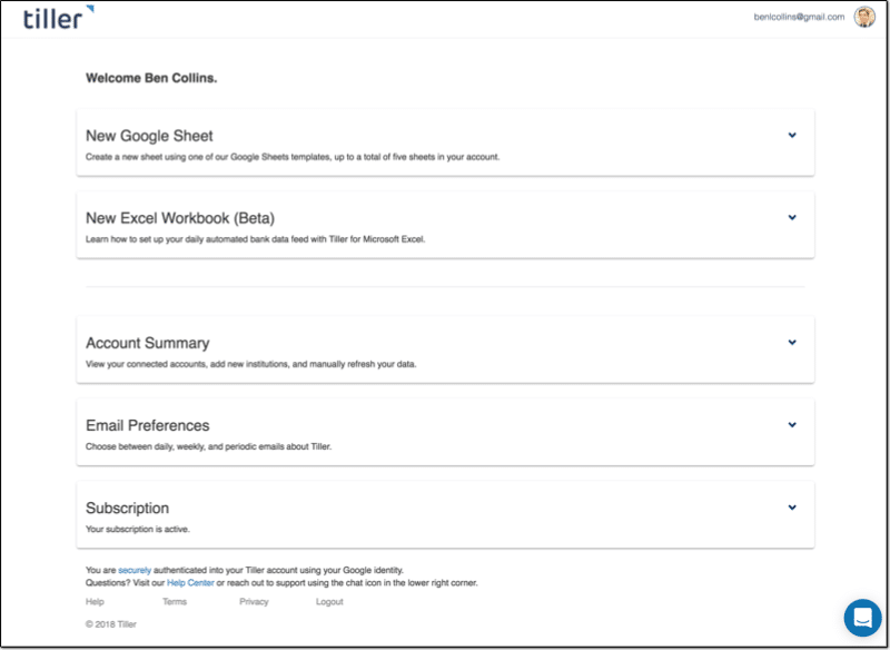
Tiller is a third-party tool so you have to create an account with them, which is done securely through your Google account credentials.
This is what your homepage looks like, and where you add accounts or create new Google Sheet templates:
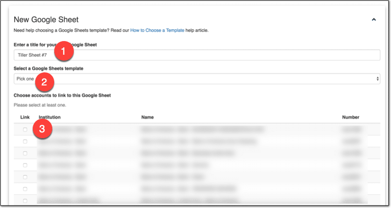
Once you add the bank accounts and credit cards you want to track, you can go ahead and create a new Google Sheet:
1. Name the Sheet 2. Choose a template or just the data 3. Select which accounts to include
Click Create and the magic happens! ?
After a short while, you can click over to your new Google Sheet, populated with all of your transaction data!
How we use Google Sheets to track our spending habits
We’ve setup categories to group our transactions, so that we can see how much we’re spending on different things at a high-level. For example, we group all restaurant expenses together into an “Eating Out” category, which allows us to see how much we spend eating out.
You want enough categories to differentiate items in a meaningful way, but not too many that you end up with too much granularity. The whole idea is to summarize transactions into something more manageable.
Each week my wife or I will jump into the Tiller Sheet and categorize any new transactions. It’s as simple as selecting the category from the drop-down menu in Transactions tab in the blank cell next to the transaction name:
You can even use Tiller’s new Autocat tool to now automatically categorize transactions for you.
Creating custom reports with Tiller and Google Sheets
I’m going to share our solution for tracking our spending habits.
It allows us to understand how we’re spending our money and identify ways to reduce it.
I created a summary table in our Tiller Google Sheet, which shows our family spending by category. It takes the data we’ve categorized in the transactions tab, which is automatically updated by Tiller, and summarizes it.
The transactions are summarized by categories in the rows, and by months across the columns. Columns A and B contain checkboxes, which I use to control which spending categories to show in my charts.
This table alone gives us more insight into our spending habits than anything the bank gives us. Every single transaction is included and categorized, by us not the bank.
In my case, I’ve used a QUERY function in cell C3 to retrieve, aggregate and pivot my transaction data:
=QUERY(QUERY(Transactions!A1:O,"select C, sum(D)*-1 group by C pivot K"),"offset 1",0)
Visualizing our spending habits in Google Sheets
I added the checkboxes in columns A and B, so there’s a way for my wife and I to choose categories to focus on.
The checkboxes can be individually checked or unchecked and they feed into other data tables that only show the data for the checked items.
Our mortgage, car lease and utility payments remain largely the same month-to-month. We know we have to pay them every month, so we don’t necessarily need to see them every time. (That’s not to say they’re not important, but trying to visualize all your categories at once will just clutter your charts to the point of being useless. )
However, seeing our discretionary spending — things like travel and eating out for example — helps us understand our spending habits and find ways to save more money in a healthy way.
We’re currently using two charts to track our spending habits:
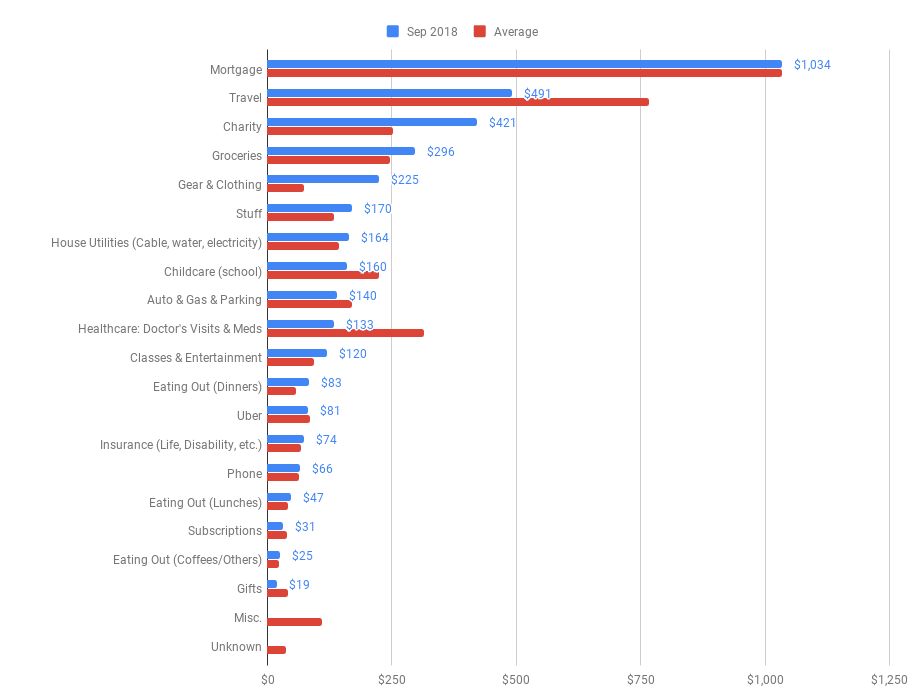
Chart 1: Current monthly spend vs. Average monthly spend
The first is a monthly breakdown by category, showing actual spend this month (blue) against the average amount we spend in this category each month (red):
(Chart shows fictional data.)
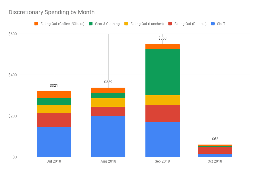
Chart 2: Discretionary Spend by Month
The second is a look at our discretionary spending over the past few months, so we can see how selected categories are trending (chart shows fictional data):
The combination of the monthly category breakdown table and these two simple charts gives us tremendous insight into our spending habits.
Knowing how we’re spending our money gives us tremendous peace of mind.
It’s helping us to minimize our unnecessary spending and maximize our saving.
Note: I’m not a financial expert and this post does not provide financial advice. It simply shows some techniques for working with and presenting data in Google Sheets.
If you use Google Sheets, or any spreadsheet application for that matter, but don’t use Pivot Tables, then you’re missing out on one of the most powerful and useful features available.
This tutorial will (attempt to) demystify Pivot Tables in Google Sheets and give you the confidence to start using them in your own work.
1. An Introduction to Pivot Tables in Google Sheets
What are Pivot Tables?
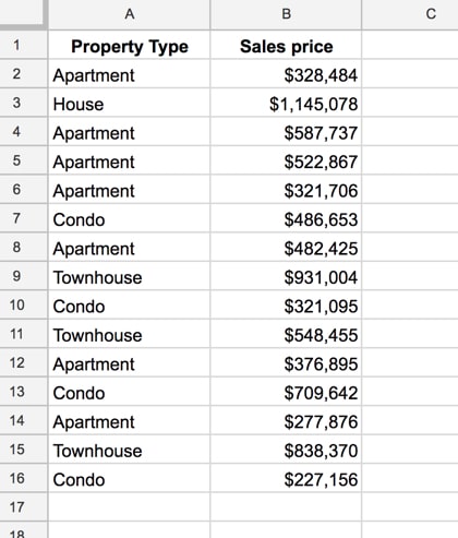
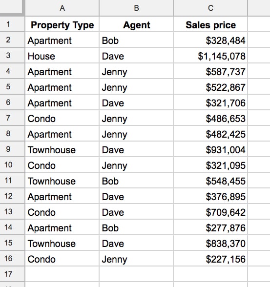
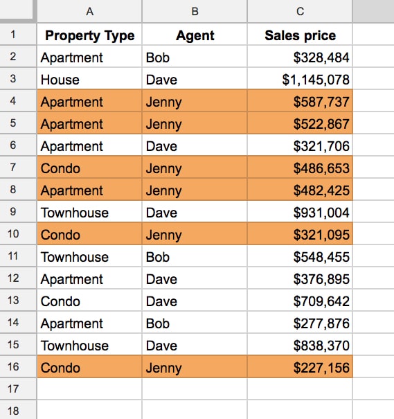
Let’s see a super simple example, to demonstrate how Pivot Tables work. Consider this dataset:
You want to summarize the data and answer questions like: how many apartments are there in the dataset? What’s the total cost of all the apartments?
Now, this would be easy to do with formulas, using a COUNTIF function and a SUMIF function, but if you change our mind and now want to summarize “Condo” you have to modify all your formulas, which is a pain.
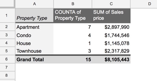
Enter the Pivot Table:
This took me eight mouse clicks and I didn’t have to write a single formula (in a few paragraphs I’ll show you those exact 8 clicks so you can build your own version).
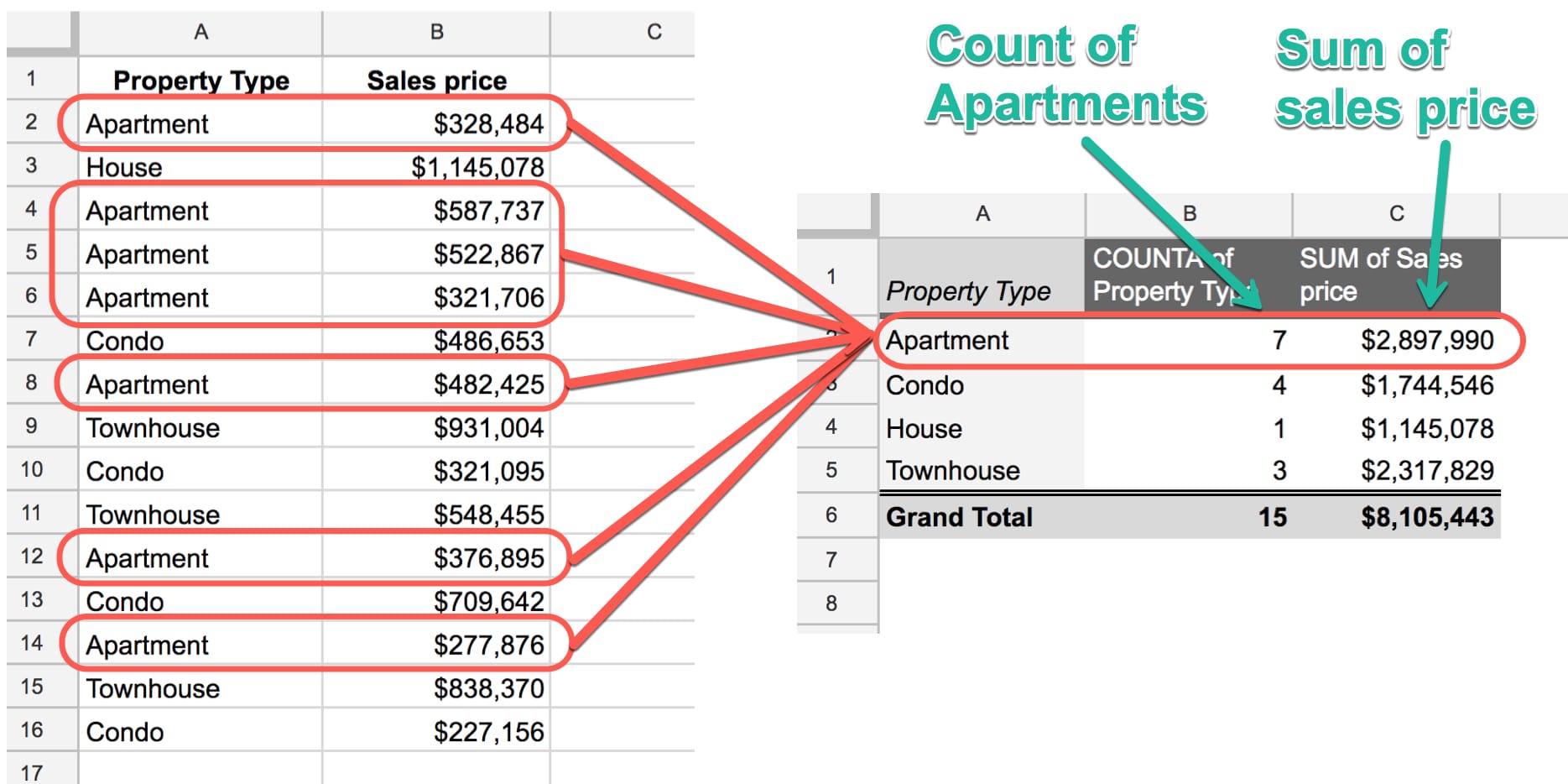
This Pivot Table summarizes the data for each property type. It counts how many of each property type is found in our dataset and then totals up the sales prices, to give a total sales price value for each property type category.
For example, the seven rows of data for Apartments are combined together into a single line in our Pivot Table (click to enlarge):
In technical parlance, the Pivot Table aggregates our data.
Pivot Tables in Google Sheets are unrivaled when it comes to analyzing your data efficiently.
They’re flexible and versatile and allow you to quickly explore your data.
Pivot Tables in Google Sheets are generally much quicker than formulas for exploring your data:
This is lesson 3 of the Pivot Tables in Google Sheets course — a comprehensive, online video course covering Pivot Tables from beginner to advanced level.
How to create your first Pivot Table
Let’s create that property type pivot table shown above. I promised you eight clicks, so here you go:
1. Copy the data from this sheet into your own blank sheet (this doesn’t count towards the 5 pivot table clicks, ok?)
2. Click somewhere inside your table of data (I’m not counting this click ?)
3. Click the menu Insert > Pivot table (clicks one and two)
This will create a new tab in your Sheet called “Pivot Table 1” (or 2, 3, 4, etc. as you create more) with the Pivot Table framework in place.
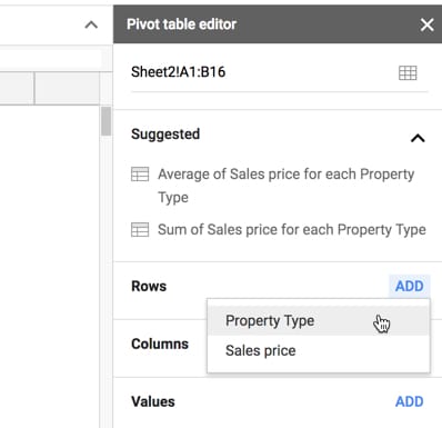
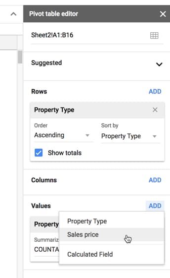
4. Click Rows in the Pivot table editor and add Property Type (clicks three and four)
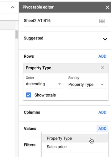
5. Click Values in the Pivot table editor and add Property Type (clicks five and six)
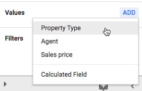
6. Click Values in the Pivot table editor and add Sales price (clicks seven and eight. Boom! ?)
Here are the steps in sequence (note that you now use Insert > Pivot table, not Data > Pivot table):
And that’s it!
Eight clicks and you have a summary report of your dataset that gives you fresh insights into your data.
Now granted this is a super simple dataset, but even if we’d had hundreds, thousands or tens of thousands of rows of data, it would still be the same eight clicks to create this Pivot Table.
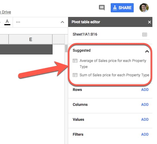
Let Google build Pivot Tables for you
Leverage the power of Google Sheets’ built-in AI!
When you create your Pivot Table, you’ll notice that Google automatically suggests some pre-built Pivot Tables for you in the editing window:
With a single click you can then create a Pivot Table:
It’s a neat way of quickly building them out as a starting point, and if it happens to answer your questions then even better.
I would absolutely still advocate learning how to build your own Pivot Tables however.
Even if you intend to always use the automatic Pivot Table builder, it’s still a good idea to understand how they work so that you know what the data is showing you.
So let’s take a look at building Pivot Tables in Google Sheets in more detail.
2. Pivot Tables in Google Sheets: Fundamentals
When you create a Pivot Table from a table of data, all of the columns from the dataset are available to use in your Pivot Tables.
Rows, columns and values
At the heart of any Pivot Table are the rows, columns and values.
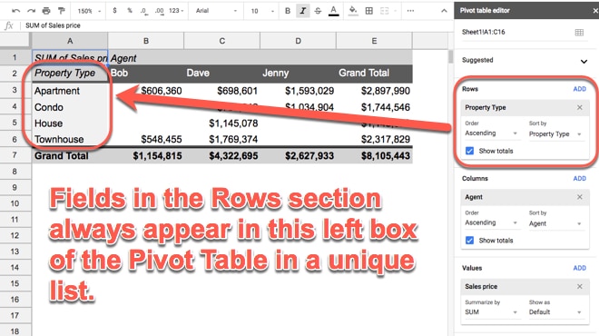
Rows:
When you click Add under the Rows, you’re presented with a list of column headings from your table. When you select one, the Pivot Table will add all of the unique items from that column into your Pivot Table as row headings. Recall from the example above, it takes all the rows of property data and squashes it down to just four rows, which are the four unique property types we see.
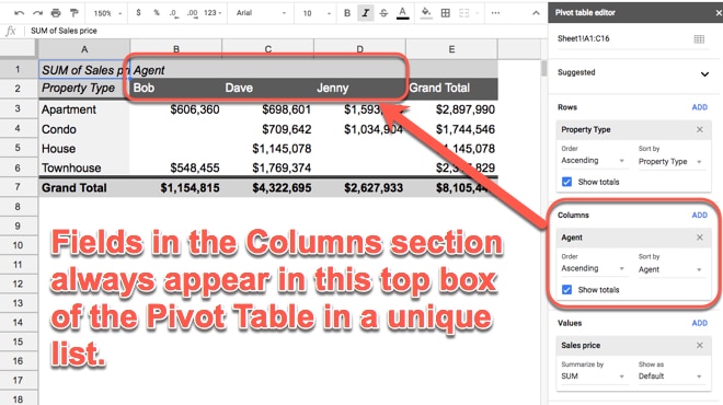
Columns:
Adding Columns produces the same effect as adding Rows, but in for the columns. The Values data is displayed in aggregated form, for each column.
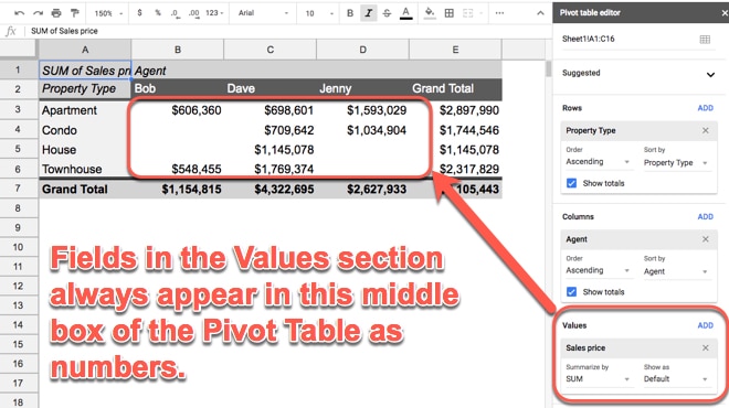
Values:
When you click on Values, you’re presented with the same list of column headings. When you select one, you’re telling the Pivot Table to summarize that column. For example, if it’s a list of revenue you might want to sum it up, or average it. Or, if it’s a column of text values, you may want to count them. This is what happens when you add values: the data is summarized, i.e. all the individual values from each row are combined together into single value (they’re aggregated).
If you have anything in the Rows section of your Pivot Table, the aggregation will be done at that level (e.g. if we have property types in Rows, the Pivot Table will display the aggregated values for each Property Type).
You can also drag-and-drop the fields in your Pivot Table to easily move them around, for example from Rows to Columns, as shown in this GIF:
Totals
You can easily toggle totals on or off for any of the Values columns in your Pivot Tables.
The button is in the Rows section:
Sorting
The sort options are found in the Rows section of your Pivot Table.
Each Row field can be used to sort with, and each one has their own sort options.
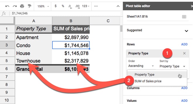
First, choose which Row field you want to sort with under the Sort by menu option (1). Then you’ll have a choice of sorting by the category field itself or any of the value fields that have been aggregated for this category column (2). This image shows this:
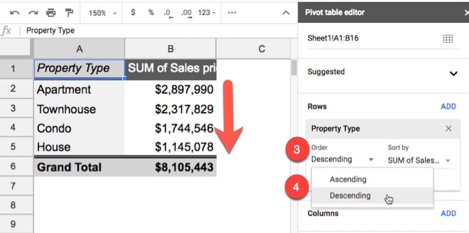
The second option for sorting data is Order (3) where you specify whether you want it ascending or descending (4):
In this example, I’ve elected to sort by the second column, the SUM of Sales Price, and then chosen to sort descending so the whole table is sorted so that the largest values in this column are at the top and the smallest values at the bottom.
3. Pivot Tables in Google Sheets: Tips and Tricks
To show you a few more tricks with Pivot Tables, we need an extra column in our data table:
So far, we’ve just looked at a single values column, showing a sum of the sales prices.
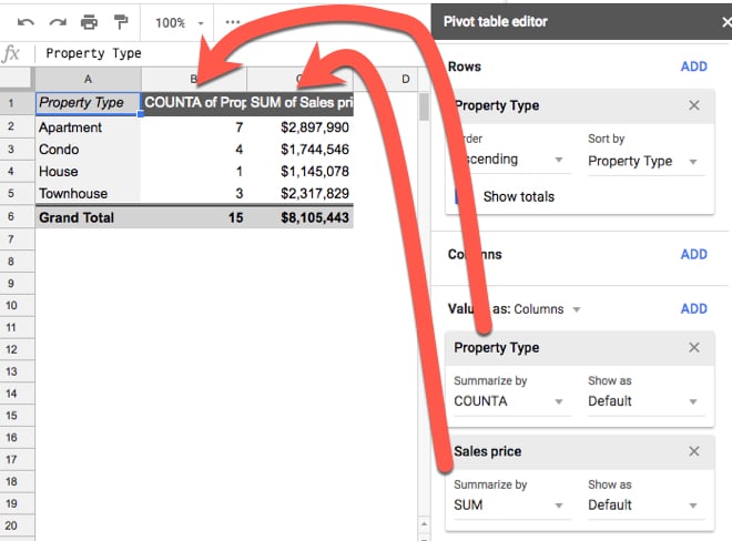
However, you can add more value columns. For example, you might want to count how many properties are in each category or what the average sales price was for each category.
Click Add in the Values section of the editor to add as many value columns as you want:
By adding the property type column (which is all the text values in our original data), the Pivot Table will default to counting the number of times each property type occurs (using the COUNTA function).
You can drag the values fields to rearrange the order of the columns in your Pivot Table.
Changing aggregation types
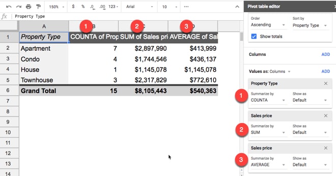
You can add the Sales Price field again, so that you have it twice in your Pivot Table. Initially it’ll default to SUM in both cases, giving you identical total columns. Not particularly useful.
However, you can change the aggregation type of one of the columns, e.g. change the SUM to AVERAGE instead, and then you’ll get fresh insights:
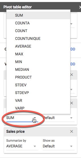
The aggregation options are accessed by clicking where its says SUM (or AVERAGE or whatever you’ve selected) and then choosing from the menu:
Pivot Table filters are conceptually the same as ordinary filters we use with our data.
We add a filter to show only a subset of our data based on some condition. For example, maybe you want to only see data from 2018, or just the month of September, or from Region A, etc.
They’re easy to add and use in Pivot Tables.
It’s the last section of the Pivot Table editor that we haven’t talked about yet.
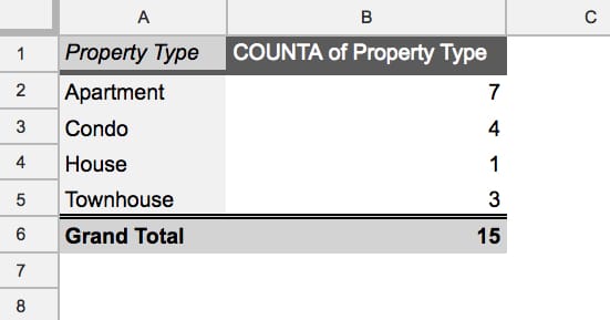
Consider this example showing a count of properties for each property type:
It shows all 15 properties from the original dataset.
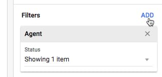
Add a filter by clicking Add in the Filter section:
In this example I’ve chosen the Agent column to add as my filter. This means that I want to choose to look at the data from just one of the Agents in my Pivot Table, i.e. filter down to show only that Agent’s data.
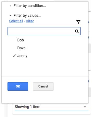
To filter on Jenny only for example, click on the “Status > Showing all items” and uncheck the items you want to discard. Whatever is left selected (shown with a tick) is the data that will be used to create the Pivot Table.
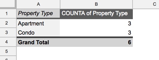
The output shows only the six properties for which Jenny was the agent:
Looking back at the data, what’s happening is that the Pivot Table is only including the rows of data related to Jenny in the Pivot Table, i.e. these six rows:
Multiple categories
(Note: I’ve taken off the filter for this exercise.)
What happens when we add multiple fields to our Rows section? Let’s see.
The first field you add shows creates a unique list of items from that column. When you add a second row field, it appears as sub-categories, so that between the two columns in your Pivot Table, all the unique combinations of the two fields are shown.
Swapping the order of the row fields, by simply dragging and dropping them in the Pivot Table editor window, will swap the order of the categories.
For example, you can summarize the breakdown of property types for each Agent, or you can summarize the sales by each Agent for each Property Type.
Like everything with Pivot Tables don’t be afraid to just experiment here. Try different combinations and take a moment to understand what the Pivot Table is showing with each combination.
Copying Pivot Tables in Google Sheets
Oftentimes you’ll find yourself wanting to replicate a Pivot Table, perhaps as a starting point for further data exploration.
There’s a quick trick for copying an existing Pivot Table, rather than starting over. It also gives you the option of moving your Pivot Tables to a different tab.
Click into the top left corner cell of your Pivot Table and click copy (Cmd + C on a Mac, or Ctrl + C on a PC/Chromebook). This adds the Pivot Table to your clipboard and you can paste it wherever you want in your Sheet (Cmd + V on a Mac, or Ctrl + V on a PC/Chromebook).
Note: You need to ensure there is enough space available wherever you wish to paste a copy of your Pivot Table (i.e. enough empty cells) or you’ll see the #REF! error.
Extracting Data from Pivot Tables
To extract data correctly from pivot tables, use the GETPIVOTDATA function. Regular cell references can lead to errors if the pivot table changes size.
4. Pivot Tables: Next steps
The nice thing with Pivot Tables in Google Sheets is that they’re really easy to experiment with. Just try adding different fields in different parts of your Pivot table editor to see what effect it has. You can always start over!
+ Check out my online training course, Pivot Tables in Google Sheets course, for a complete look at Pivot Tables, from beginner through to advanced level.
+ Keep up-to-date with new articles, course launches and exclusive offers, by signing up for my Google Sheets newsletter, and get my free 80-page ebook on Google Sheets tips.
Let me show you a unique use case for pivot tables – Pivot Table Maps!
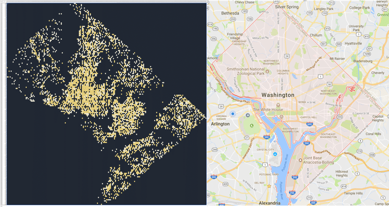
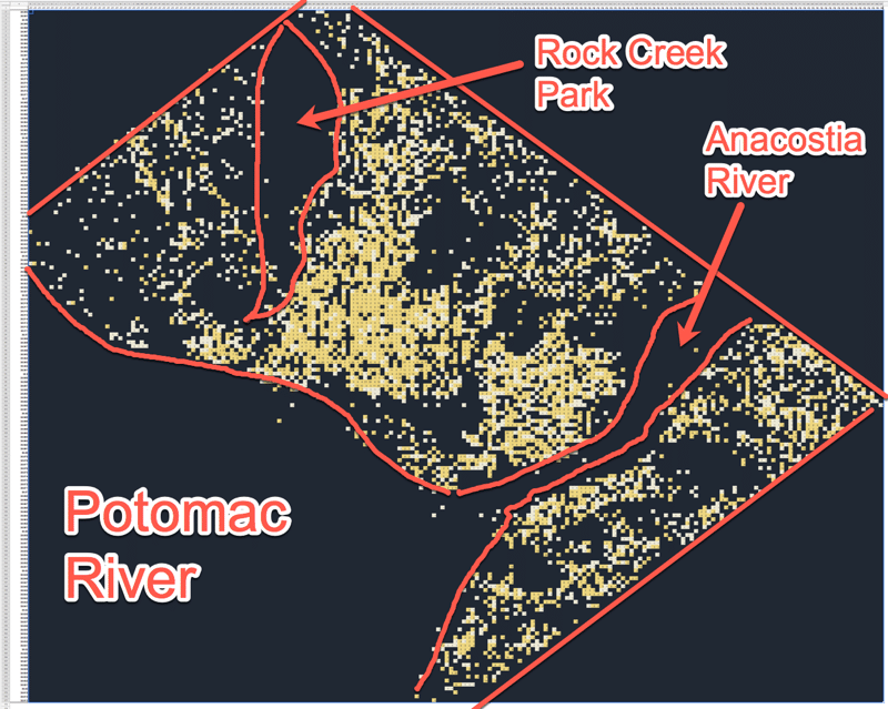
Can you guess which city this is?
It’s Washington D.C. and it’s also a pivot table in Google Sheets. The image on the left is the Pivot Table map built with a pivot table. The image on the right is a screenshot of Washington D.C. from Google maps.
Look closely and you might just be able to see the Google Sheet row and column headings around the map.
Wait, what?
I downloaded a dataset of DC crime data, which had latitude and longitude data, and plotted it as a pivot table with conditional formatting.
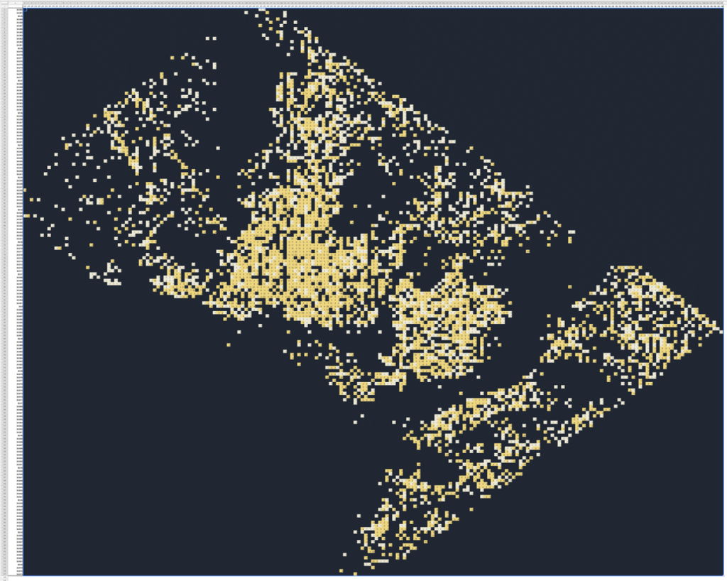
The dark areas in the pivot table map represent Rock Creek Park (huge wooded area with few people, hence few crimes) and two rivers, the Anacostia, which runs through the SE of the city, and the Potomac river, which delineates the W edge of the city.
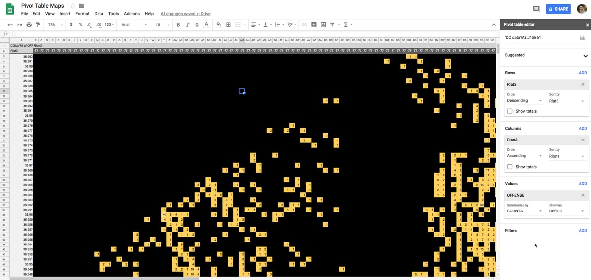
And here’s a close up of the Sheet, to convince you it’s really a pivot table (click to enlarge) 😉
I first saw this technique implemented in Excel (see this example) but I haven’t seen anything in Google Sheets before.
How to make Pivot Table Maps
It’s actually pretty simple and can be performed on any dataset with latitude and longitude data, to varying degrees of success (some datasets are too large, some not granular enough).
Download your chosen dataset.
Round your latitude and longitude data columns to 1, 2 or 3 decimal places (depending on how granular your data is, trial and error).
Highlight the whole data table and create a pivot table.
Insert latitude as rows.
Sort the latitude rows as descending, since larger positive numbers are further North.
Insert longitude as columns.
Highlight all the longitude columns and reduce the column width of all of them in one go, so all the cells are square.
Insert your measure into the values section of your pivot report builder, in the DC map example above I inserted “Offense” and used COUNTA to count them.
Highlight whole pivot table and choose Conditional Formatting –> Color Scale (I chose variations of yellow).
Change the background of the pivot table to black.
Zoom out on your Sheet as far as you need to see the full “map”.
It’s a quick and dirty way of visualizing geographic data sets.
It’s not really suitable for deep analysis or final charts, where a tool like Tableau would really prove it’s worth, but for a quick look with only a few minutes work, it’s not too bad!
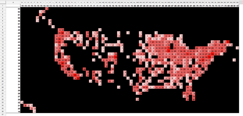
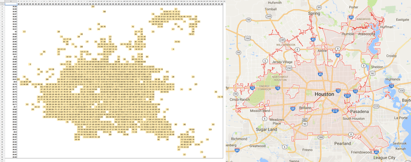
Here’s a few more Pivot Table Maps of my own:
A pivot table map of 7,000 breweries and brew pubs in the USA:
Houston, Texas as a pivot table map, created from 311 data:
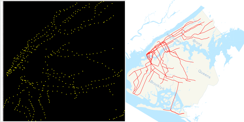
Subway stations of New York City pivot table map:
Let me know if you try this yourself! I’d love to see any creations you come up with.