Slicers in Google Sheets are a powerful way to filter data in Pivot Tables.
They make it easy to change values in Pivot Tables and Charts with a single click. Slicers are extremely useful when building dashboards in Google Sheets.
Educator and Google Developer Expert. Helping you navigate the world of spreadsheets & AI.
Slicers in Google Sheets are a powerful way to filter data in Pivot Tables.
They make it easy to change values in Pivot Tables and Charts with a single click. Slicers are extremely useful when building dashboards in Google Sheets.
The Google Sheets Filter function is a powerful function we can use to filter our data. The Google Sheets Filter function will take your dataset and return (i.e. show you) only the rows of data that meet the criteria you specify (e.g. just rows corresponding to Customer A).
Suppose we want to retrieve all values above a certain threshold? Or values that were greater than average? Or all even, or odd, values?
The Google Sheets Filter function can easily do all of these, and more, with a single formula.
This video is lesson 13 of 30 from my free Google Sheets course: Advanced Formulas 30 Day Challenge.
In this example, we have a range of values in column A and we want to extract specific values from that range, for example the numbers that are greater than average, or only the even numbers.
The filter formula will return only the values that satisfy the conditions we set. It takes two arguments, firstly the full range of values we want to filter and secondly the conditions we’re going to apply. The syntax is:
=FILTER("range of values", "condition 1", ["condition 2", ...])where Condition 2 onwards are all optional i.e. the Filter function only requires 1 condition to test but can accept more.
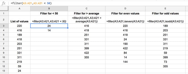
For example in the image above, here are the conditions and corresponding formulas:
| Conditions | Formula |
| Filter for < 50 |
=filter(A3:A21,A3:A21<50)
|
| Filter for > average |
=filter(A3:A21,A3:A21>AVERAGE(A3:A21))
|
| Filter for even values |
=filter(A3:A21,iseven(A3:A21))
|
| Filter for odd values |
=filter(A3:A21,isodd(A3:A21))
|
The results are as follows:
(Note: not all the values are shown in column A.)
Absolutely!
For example, using the basic data above, we could display all the 200-values (i.e. values between 200 and 300) with this formula:
=FILTER(A3:A21, A3:A21>200, A3:A21<300)Yes, simply add them as additional criteria to test. For example in the following image there are two columns of exam scores. The Filter function used returns all the rows where the score is over 50 in both columns:
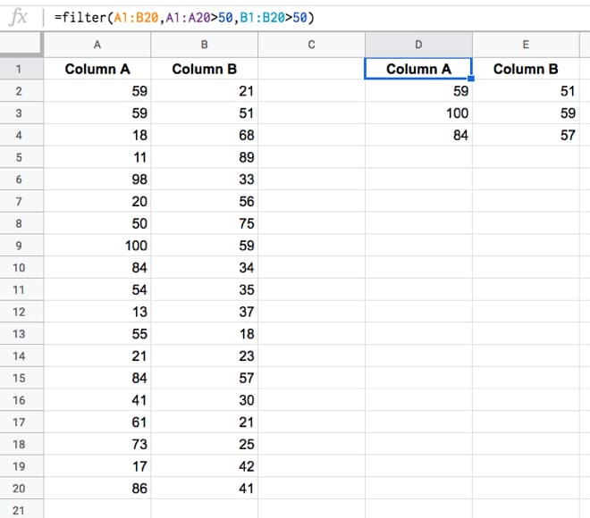
The formula is:
=FILTER(A1:B20,A1:A20 > 50,B1:B20 > 50)Note, using the Filter function with multiple columns like this demonstrates how to use AND logic with the Filter function. Show me all the data where criteria 1 AND criteria 2 (AND criteria 3...) are true.
For OR logic, have a read of this post: Advanced Filter Examples in Google Sheets
Instead of hard-coding a value in the criteria, you can simply reference another cell which contains the test criteria. That way you can easily change the test criteria or use other parts of your spreadsheet analysis to drive the Filter function.
For example, in this image the Filter function looks to cell E1 for the test criteria, in this case 70, and returns all the values that exceed that score, i.e. everything over 70.
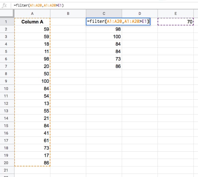
The formula in this example is:
=FILTER(A1:A20,A1:A20 > E1)Yes, you can!
Use the output of your first filter as the range argument of your second filter, like this:
=FILTER( FILTER( range, conditions ), conditions )Advanced Filter Examples in Google Sheets
Google documentation for the FILTER function.
 Advanced Filter Examples in Google Sheets
 Google Sheets Query function: The Most Powerful Function in Google Sheets
In this post we’ll look at how to calculate a running total, using a standard method and an array formula method. We’ll cover the topic of matrix multiplication (take a deep breath, it’s going to be ok!) using the MMULT formula, one of the more exotic, and challenging formulas in Google Sheets.
If you like video tutorials, here’s the one on MMULT:
This is a lesson from my latest, Google Sheets course on Advanced Formulas 30 Day Challenge (it’s free!).
Continue reading Running Total Array Formulas Using The MMULT Function
It probably won’t surprise you to hear that I use a Google Sheets budget template to track my finances, both incomings and outgoing, at home and for my business.
The dashboards available through online banking sites are pretty rudimentary. They don’t give much insight into what’s happening with my finances, particularly over longer time frames.
I like using Google Sheets, as opposed to another third party service like Mint, because it’s fully customizable. It’s easy to use and I can share any spending or budget templates easily with my wife.
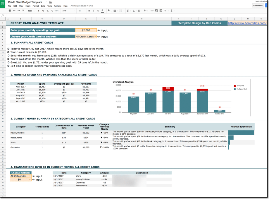
I’m not a financial expert, so I won’t be dispensing any financial advice here. I won’t opine on what you should or shouldn’t show in your spending and budget templates in this post, nor will I talk about what your financial goals should be or how to get there.
What I will do in this post however, is show you some useful tips in Google Sheets that you can use for building your own budget templates. Techniques to make them more insightful and more helpful for reaching your goals.
Continue reading 10 Tips To Build A Google Sheets Budget Template
This post shows you how to connect a Google Sheet to GitHub’s API, with Oauth and Apps Script. The goal is to retrieve data and information from GitHub and show it in your Google Sheet, for further analysis and visualization.
If you manage a development team or you’re a technical project manager, then this could be a really useful way of analyzing and visualizing your team’s or project’s coding statistics against goals, such as number of commits, languages, people involved etc. over time.
Note, this is not a post about integrating your Apps Script environment with GitHub to push/pull your code to GitHub. That’s an entirely different process, covered in detail here by Google Developer Expert Martin Hawksey.
Continue reading Show data from the GitHub API in Google Sheets, using Apps Script and Oauth