In this post, you’ll see how to highlight duplicates in Google Sheets and how to remove duplicates in Google Sheets.
Duplicates are instances of the same record appearing in your data more than once.
They’re a huge problem and it’s critical to find duplicates in Google Sheets before any data analysis is performed.
Imagine you had two instances of the same client transaction for $5,000 in your database. When you summarize your data, you might think you have $10,000 in revenue from that client when in fact you only have $5,000. You’ll make decisions based on the wrong data.
Contents
- Method 1: How to remove duplicates with the Remove Duplicates tool
- Method 2: How to remove duplicates with formulas
- Method 3: How to find duplicates with Pivot Tables
- Method 4: How to highlight duplicates with Conditional Formatting
- Method 5: How to remove duplicates with Apps Script
However, here’s a rundown of when to use the different methods:
Method 1: Remove Duplicates tool is the easiest method of removing duplicates.
Method 2: Formulas The UNIQUE function is great for small, simple datasets or when you need to remove duplicates inside a nested formula.
Method 3: Pivot Tables are a great way to highlight duplicates in Google Sheets. Pivot Tables are extremely flexible and fast to use, so they’re a great tool to use when you’re unsure if you have duplicates and want to check your data.
Method 4: Conditional Formatting is a great way to highlight duplicates in Google Sheets.
Method 5: Apps Script is useful for developers who want to remove duplicates from Sheets as part of their apps, or someone who needs to repeatedly and automatically de-duplicate their data.
Method 1: How to remove duplicates in Google Sheets with the Remove Duplicates tool
The new feature is super easy to use. You find this feature under the menu:
Data > Data cleanup > Remove Duplicates
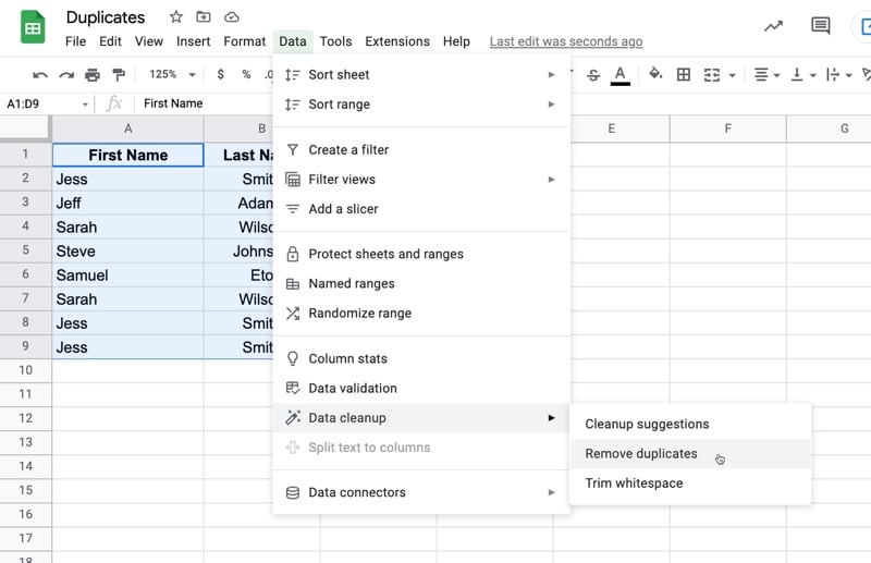
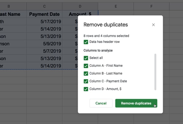
When you click Remove Duplicates, you’ll be prompted to choose which columns you want to check for duplicates.
You may want to remove duplicates where the rows entirely match, or you may wish to choose a specific column, such as an invoice number, regardless of what data is in the other columns.
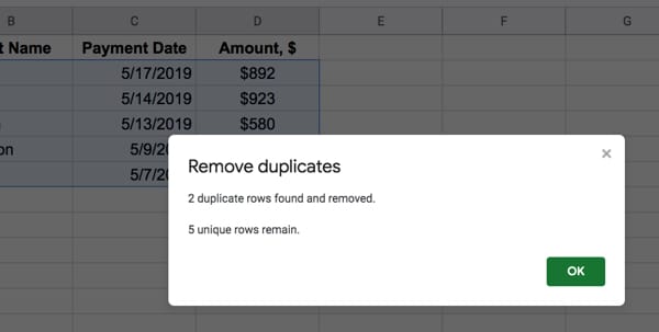
The duplicates will then be removed and you’ll be presented with a summary report, telling you how many duplicates were removed:
Method 2: How to remove duplicates in Google Sheets using formulas
2.1 Use the UNIQUE formula
This method deletes duplicates in the range of data you select.
The UNIQUE function considers all the columns of your data range when determining the duplicates. In other words, it compares each row of data and removes any rows that are duplicates (identical to any others across the whole row).
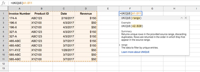
It’s very easy to implement as it involves a single formula with a single argument — the range you want to de-duplicate (remove duplicates from).
=UNIQUE(A1:D11)
Here’s an example of the UNIQUE function in action. The function is in cell F1 and looks for duplicates in the data range in A1:D11:
And this is the result:
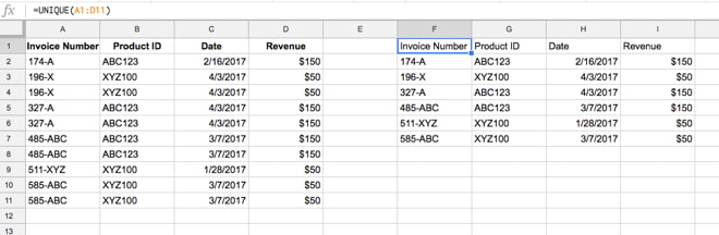
You can see the table on the right has fewer rows, because the duplicate rows have been removed.
2.2 Highlight duplicate values with COUNTIF
This method uses the COUNTIF function to highlight duplicates in Google Sheets.
First, create a new column next to the data column you want to check for duplicates (e.g. invoice number).
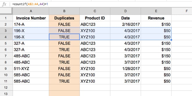
Then use this formula in cell B2 to highlight the duplicates in column A:
=COUNTIF(A$2:A2,A2)>1
You’ll notice the range is A$2:A2
The $ sign is key here because it locks the range to the top of the column, even as you copy the formula down column B. So this formula checks for duplicates in the current row back up to the top.
When a value shows up for the first time, the count will be 1, so the formula result will be false. But when the value shows up a second time, the count will be 2, so the formula result will be TRUE.
The final step is to select the rows with TRUE values (the duplicates) and delete them.
Note: If you have a large dataset, with a lot of duplicates, then it’s best to turn the Duplicate column into values (Copy > Paste Special), sort by this column so all the duplicates (TRUEs) are in a block at the bottom of your dataset, and then delete them in one big group. It’s much quicker.
Method 3: How to find duplicates in Google Sheets using Pivot Tables
If you’re new to Pivot Tables, check out my article Pivot Tables 101: A Beginner’s Guide.
Pivot Tables are a great tool to use to search for duplicates in Google Sheets. They’re extremely flexible and fast to use, so they’re often a great place to start if you’re unsure whether you have any duplicates in your data.
Step 1:
Highlight your dataset and create a Pivot Table (under the Data menu).
A new tab opens with the Pivot Table editor.
Step 2:
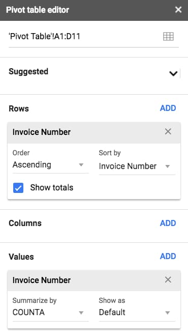
Under ROWS, choose the column you want to check for duplicates (e.g. invoice number).
Step 3:
Then in VALUES, choose another column (I often use the same one) and make sure it’s set to summarize by COUNT or COUNTA (if your column contains text), like this:
The Pivot Table will then look like this:
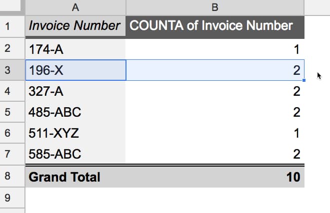
You can see that duplicates values (for example 196-X) will have a count greater than 1.
From here you can find these duplicate values in your original dataset and decide how to proceed.
As you can see, this method is most suitable to find duplicates in Google Sheets.
Method 4: How to highlight duplicates in Google Sheets using Conditional Formatting
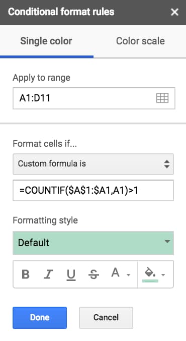
Select your dataset and open the conditional formatting sidebar (under the Format menu).
Under the “Format cells if…” option, choose custom formula is (the last option) and enter the following formula:
=COUNTIF($A$1:$A1,A1)>1
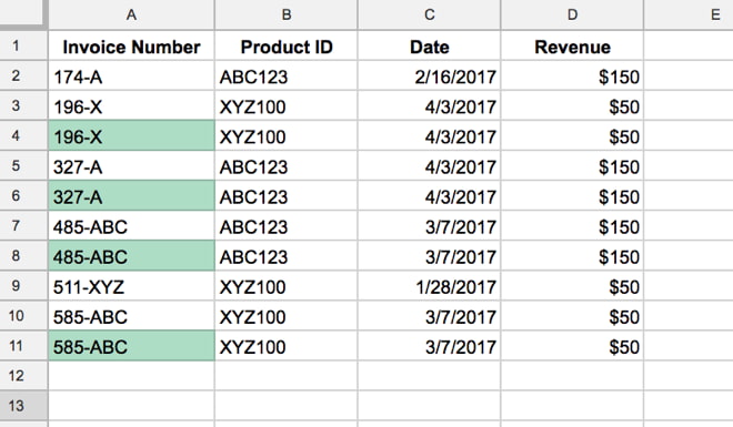
This formula checks for duplicates in a single column only, in this case column A.
The output is highlighting applied to the duplicate values:
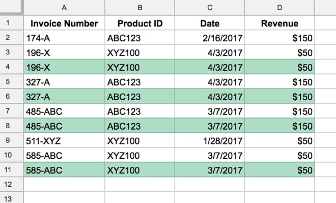
What if you want to apply the highlight to the whole row?
You need to make one small tweak to the formula (highlighted in red) by adding a $ sign in front of the final A:
=COUNTIF($A$1:$A1,$A1)>1
Now your output will look like this, with the whole row highlighted:
Check out this article for a more detailed look at how to highlight a whole row using conditional formatting.
Method 5: How to remove duplicates in Google Sheets using Apps Script
(New to Apps Script? Read my starter guide to Apps Script for a primer.)
It’s relatively straightforward to create a small script file that can remove duplicate rows from your datasets.
The advantage of writing an Apps Script program is that you can run it over and over, for example each time you add new data.
Sample Apps script program: How to remove duplicates in Google Sheets
This program removes duplicates from a dataset in Sheet 1. It’s very specific to the Sheet and data range, but it’s easy to create and modify.
It works as follows:
- Get the values from the data range in Sheet1, using Apps Script
- Turn the array rows into strings (blocks of text) for comparison
- Filter out any duplicate rows
- Check whether a de-duplicate sheet exists
- If it does, clear out the old data and paste in the new de-duplicated data
- If it does not exist, create a new sheet and paste in the new de-duplicated data
- Add a custom menu to run from the Google Sheet
So it’s very specific to this use case, but it could be easily adapted if necessary for different datasets. Here it is in action:
And here’s the Apps Script code for this program:
/**
* remove duplicate rows from Google Sheets data range
*/
function removeDupRows() {

  var ss = SpreadsheetApp.getActiveSpreadsheet();
  var sheet = ss.getSheetByName('Sheet1');

  // change the row number of your header row
  var startRow = 7;

  // get the data
  var range = sheet.getRange(startRow,1,sheet.getLastRow(),sheet.getLastColumn()).getValues();

  // remove duplicates with helper function
  var dedupRange = arrayUnique(range);
  Logger.log(dedupRange);

  // check if duplicate sheet exists already, if not create new one
  if (ss.getSheetByName('Sheet1 Duplicates Removed')) {

    // case when dedup sheet already exists
    var dedupSheet = ss.getSheetByName('Sheet1 Duplicates Removed');
    var lastRow = Math.max(dedupSheet.getLastRow(),1);
    var lastColumn = Math.max(dedupSheet.getLastColumn(),1);

    // clear out any previous de-duplicate data
    dedupSheet.getRange(1,1,dedupSheet.getLastRow(),dedupSheet.getLastColumn()).clear();

    // replace with new de-duplicated data
    dedupSheet.getRange(1,1,dedupRange.length,sheet.getLastColumn()).setValues(dedupRange);
  }
  else {

    // case when there is no dedup sheet
    var dedupSheet = ss.insertSheet('Sheet1 Duplicates Removed',0);
    dedupSheet.getRange(1,1,dedupRange.length,dedupRange[0].length).setValues(dedupRange);
  }

  // make the de-duplicate sheet the active one
  dedupSheet.activate();

}

/**
* helper function returns unique array
*/
function arrayUnique(arr) {

  var tmp = [];

  // filter out duplicates
  return arr.filter(function(item, index){

    // convert row arrays to strings for comparison
    var stringItem = item.toString();

    // push string items into temporary arrays
    tmp.push(stringItem);

    // only return the first occurrence of the strings
    return tmp.indexOf(stringItem) >= index;

  });
}
And you can also add a custom menu to run it from your Google Sheet rather than the script editor window:
/**
* add menu to run function from Sheet
*/
function onOpen() {
  var ui = SpreadsheetApp.getUi();
  ui.createMenu('Remove duplicates')
  .addItem('Highlight duplicate rows','highlightDupRows')
  .addItem('Remove duplicate rows','removeDupRows')
  .addToUi();
}
The code for this simple duplicate program is also here on GitHub.
Suggestions for improvement
- Set triggers to run the duplicate remover on certain conditions (e.g. once a day, when new data is added)
- Better control over selecting the data (i.e. which Sheet, what range etc.)
- Whether to consider all of the columns or not for duplicates
- Better control over the output
I started coding something along these lines, but it gets complicated as you start to pile on more edge-cases and user options. I realized pretty quickly that all I was doing was reinventing the wheel, since a perfectly fine tool exists already (the built-in one!).
The best thing about Apps Script is that it lets you build minimal viable products specific to your situation very quickly.
Once you’re familiar with Apps Script, it only takes 15 – 30 minutes to build custom scripts, like this one to remove duplicates in Google Sheets.
Now you know how to remove duplicates in Google Sheets with five different techniques, go forth and banish those duplicates from your datasets!