This tutorial is written for Google Sheets users who have datasets that are too big or too slow to use in Google Sheets. It’s written to help you get started with Google BigQuery.
If you’re experiencing slow Google Sheets that no amount of clever tricks will fix, or you work with datasets that are outgrowing the 10 million cell limit of Google Sheets, then you need to think about moving your data into a database.
As a Google user, probably the best and most logical next step is to get started with Google BigQuery and move your data out of Google Sheets and into BigQuery.
By the end of this tutorial, you will have created a BigQuery account, uploaded a dataset from Google Sheets, written some queries to analyze the data and exported the results back to Google Sheets to create a chart.
You’ll also do the same analysis side-by-side in a Google Sheet, so you can understand exactly what’s happening in BigQuery.
I’ve highlighted the action steps throughout the tutorial, to make it super easy for you to follow along:
Google BigQuery exercise steps are shown in blue.
Actions for you to do in Google BigQuery.
Google Sheet exercise steps are shown in green.
Actions for you to do in Google Sheets.
Section 1: What is BigQuery?
Google BigQuery is a data warehouse for storing and analyzing huge amounts of data.
Officially, BigQuery is a serverless, highly-scalable, and cost-effective cloud data warehouse with an in-memory BI Engine and machine learning built in.
This is a formal way of saying that it’s:
Works with any size data (thousands, millions, billions of rows…)
Easy to set up because Google handles the infrastructure
Grows as your data grows
Good value for money, with a generous free tier and pay-as-you-go beyond that
Lightning fast
Seamlessly integrated with other Google tools, like Sheets and Data Studio
Can import and export data from and to many sources
Has Built-in machine learning, so predictive modeling can be set up quickly
What’s the difference between BigQuery and a “regular” database?
BigQuery is a database optimized for storing and analyzing data, not for updating or deleting data.
It’s ideal for data that’s generated by e-commerce, operations, digital marketing, engineering sensors etc. Basically, transactional data that you want to analyze to gain insights.
A regular database is suitable for data that is stored, but also updated or deleted. Think of your social media profile or customer database. Names, emails, addresses, etc. are stored in a relational database. They frequently need to be updated as details change.
Section 2: Google BigQuery Setup
It’s super easy to get started wit Google BigQuery!
There are two ways to get started: 1) use the free sandbox account (no billing details required), or 2) use the free tier (requires you to enter billing details, but you’ll also get $300 free Cloud credits).
In either case, this tutorial won’t cost you anything in BigQuery, since the volume of data is so tiny.
We’ll proceed using the sandbox account, so that you don’t have to enter any billing details.
A new project called “My First Project” is automatically created
In the left side pane, scroll down until you see BigQuery and click it
Here’s that process shown as a GIF:
You’re ready for Step 2 below.
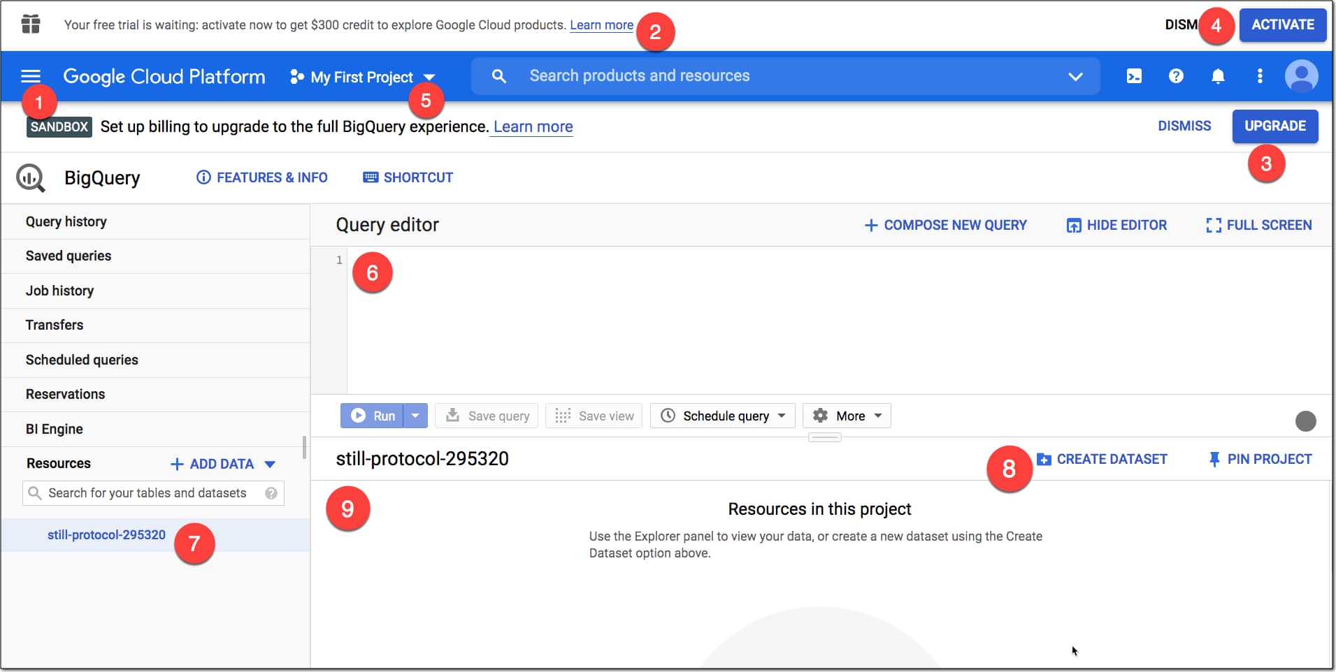
BigQuery Console
(click to enlarge)
Here’s what you can see in the console:
The SANDBOX tag to tell you you’re in the sandbox environment
Message to upgrade to the free trial and $300 credit (may or may not show)
UPGRADE button to upgrade out of the Sandbox account
ACTIVATE button to claim the free $300 credit
The current project and where to create new projects
The Query editor window where you type your SQL code
Current project resource
Button to create a new dataset for this project (see below)
Query outputs and table information window
What is the free Sandbox Account?
The sandbox account is an option that lets you use BigQuery without having to enter any credit card information. There are limits to what you can do, but it gives you peace of mind that you won’t run up any charges whilst you’re learning.
In the sandbox account:
Tables or views last 60 days
You get 10 Gb of storage per month for free
And 1 Tb data processing each month
It’s more than enough to do everything in this tutorial today.
Unlike Google Sheets, you have to pay to use BigQuery based on your storage and processing needs.
However, there is a sandbox account for free experimentation (see below) and then a generous free tier to continue using BigQuery.
In fact, if you’re working with datasets that are only just too big for Sheets, it’ll probably be free to use BigQuery or very cheap.
BigQuery charges for data storage, streaming inserts, and for querying data, but loading and exporting data are free of charge.
Your first 1 TB (1,000 GB) per month is free.
Full BigQuery pricing information can be found here.
Clicking on the blue “Try BigQuery free” button on the BigQuery homepage will let you register your account with billing details and claim the free $300 cloud credits.
Section 3: How to get your data into BigQuery
Extracting, loading and transforming (ELT) is sometimes the most challenging and time consuming part of a data analysis project. It’s the most engineering-heavy stage, where the heavy lifting happens.
You can load data into BigQuery in a number of ways:
From a readable data source (such as your local machine)
From Google Sheets
From other Google services, such as Google Ad Manager and Google Ads
Use a third-party data integration tool, e.g. Supermetrics, Stitch
You might want to make a SECOND copy in your Drive folder too, so you can keep one copy untouched for the upload to BigQuery and use the second copy for doing the follow-along analysis in Google Sheets.
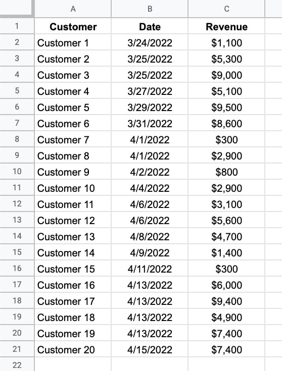
The first dataset is a record of pedestrian traffic crossing Brooklyn Bridge in New York city (source).
It’s only 7,000 rows, so it could be easily analyzed in Sheets of course, but we’ll use it here so that you can do the same steps in BigQuery and in Sheets.
The second dataset is a daily total of bike counts for New York’s East River bridges (source).
There’s nothing inherently wrong with putting “small” data into BigQuery. Yes, it’s designed for truly gigantic datasets (billions of rows+) but it works equally well on data of any size.
Back in the BigQuery Console, you need to set up a project before you can add data to it.
Get started with Google BigQuery: Loading data From A Google Sheet
Think of the Project as a folder in Google Drive, the Dataset as a Google Sheet and the Table as individual Sheet within that Google Sheet.
The first step to get started with Google BigQuery is to create a project.
In step 1, BigQuery will have automatically generated a new project for you, called “My First Project”.
If it didn’t, or you want to create another new project, here’s how.
Step 3: Create a new Project
In the top bar, to the right of where it says “Google Cloud Platform”, click on Project drop-down menu.
In the popup window, click NEW PROJECT.
Give it a name, organization (your domain) and location (parent organization or folder).
Optionally, you can choose to bookmark this project in the Resources section of the sidebar. Click “PIN PROJECT” to do this.
Step 4: Create a new Dataset
Next you need to create a dataset by clicking “CREATE DATASET“.
Name it “start_bigquery”. You’re not allowed to have any spaces or special characters apart from the underscore.
Set the data location to your locale, leave the other settings alone and then click “Create dataset”
This new dataset will show up underneath your project name in the sidebar.
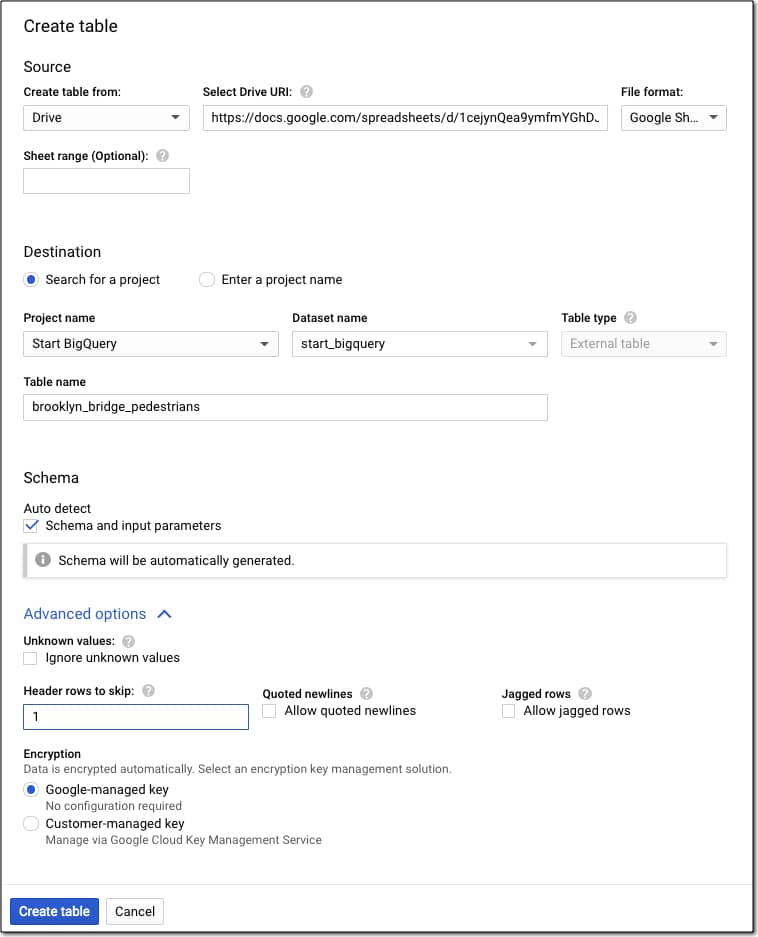
Step 5: Create a new Table
With the dataset selected, click on the “+ CREATE TABLE” or big blue plus button.
You want to select “Drive”, add the URL and set the file format to Google Sheets.
Name your table “brooklyn_bridge_pedestrians”.
Choose Auto detect schema.
Under Advanced settings, tell BigQuery you have a single header row to skip by entering the value 1.
Your settings should look like this:
If you make a mistake, you can simply delete the table and start again.
Section 4: Analyzing Data in BigQuery
Google BigQuery uses Structure Query Language (SQL) to analyze data.
The Google Sheets Query function uses a similar SQL style syntax to parse data. So if you know how to use the Query function then you basically know enough SQL to get started with Google BigQuery!
Basic SQL Syntax for BigQuery
The basic SQL syntax to write queries looks like this:
SELECT these columns
FROM this table
WHERE these filter conditions are true
GROUP BY these aggregate conditions
HAVING these filters on aggregates
ORDER BY i.e. sort by these columns
LIMIT restrict answer to X number of rows
You’ll see all of these keywords and more in the exercises below.
Get started with Google BigQuery: First Query
The BigQuery console provides a button that gives you a starter query.
Step 6: Write your first query
Click on “QUERY TABLE” and this query shows up in your editor window:
SELECT FROM `start-bigquery-294922.start_bigquery.brooklyn_bridge_pedestrians` LIMIT 1000
Modify it by adding a * between the SELECT and FROM, and reducing the number after LIMIT to 10:
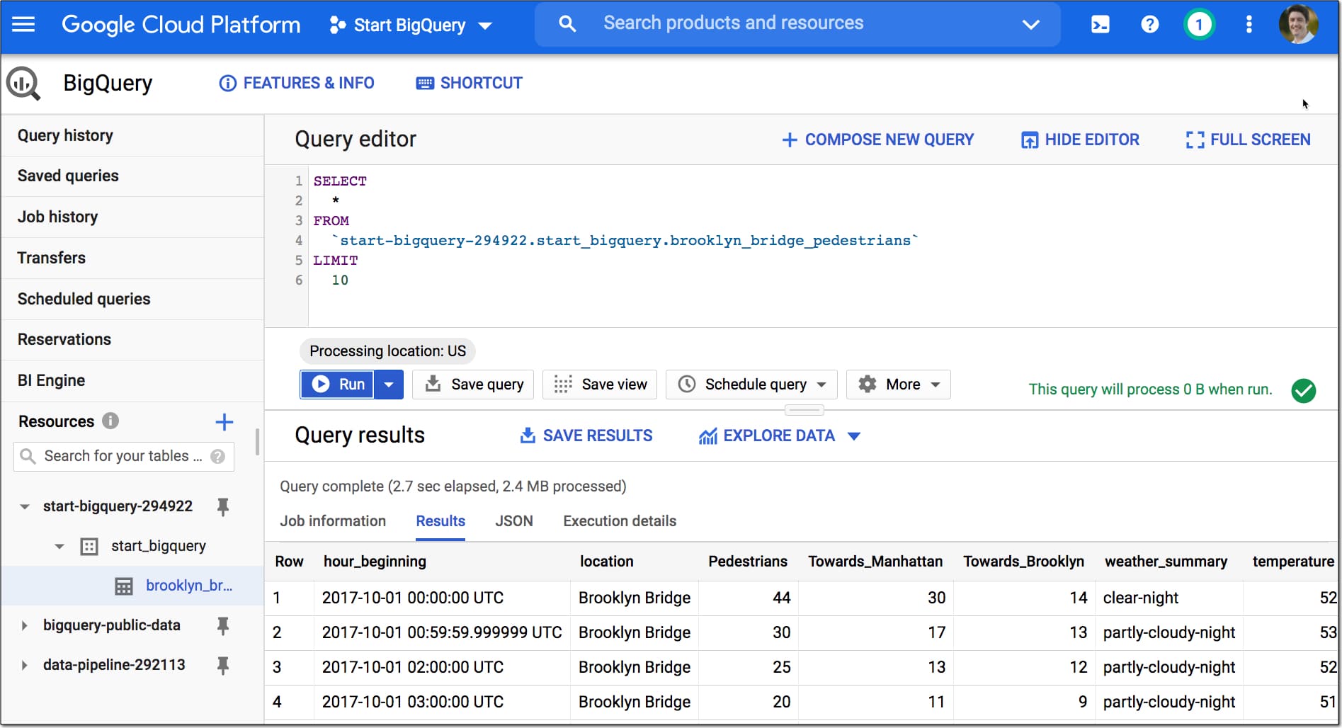
SELECT
  *
FROM
  `start-bigquery-294922.start_bigquery.brooklyn_bridge_pedestrians`
LIMIT
  10
Then format your query across multiple lines with through the menu: More > Format
SELECT
*
FROM
`start-bigquery-294922.start_bigquery.brooklyn_bridge_pedestrians`
LIMIT
10
Click “▶️ Run” to execute the query.
The output of this query will be 10 rows of data showing under the query editor:
(click to enlarge)
Woohoo!
You just wrote your first query in Google BigQuery.
Let’s continue and analyze the dataset:
Exercise 2: Analyzing Data In BigQuery
Run through the following steps:
Step 7: tell the story of one row
I always advocate doing this with any new dataset.
Write a query that selects all the columns (SELECT *) and a limited number of rows (e.g. LIMIT 10), as you did in step 6 above.
Run that query and look at the output. Scan across one whole row. Look at every column and think about what data is stored there.
Think about doing the equivalent step in Google Sheets. Look at your dataset and scroll to the right, telling the story of a single row.
We do this step to understand our data, before getting too immersed in the weeds.
Select Specific Columns
Step 8: Select specific columns
Select specific columns by writing the column names into your query.
You can also click on column names in the schema view (click on the table name in the left sidebar to access this) to add them to the query directly.
SELECT
  hour_beginning,
  location,
  Pedestrians,
  weather_summary
FROM
  `start-bigquery-294922.start_bigquery.brooklyn_bridge_pedestrians`
LIMIT
  10
Math Operations
Let’s find out the total number of pedestrians that crossed the Brooklyn Bridge across the whole time period.
Step 9: Calculate total in Google Sheets
Open the Google Sheet you copied in Step 2, called “Copy of Brooklyn Bridge pedestrian count dataset”
Add this simple SUM function to cell C7298 to calculate the total:
=SUM(C2:C7297)
This gives an answer of 5,021,692
Let’s see how to do that in BigQuery:
Step 10: Math operations in BigQuery
Write a query with the pedestrians column and wrap it with a SUM function:
SELECT
  SUM(Pedestrians) AS total_pedestrians
FROM
  `start-bigquery-294922.start_bigquery.brooklyn_bridge_pedestrians`
This gives the same answer of 5,021,692
You’ll notice that I gave the output a new column name using the code “AS total_pedestrians“. This is similar to using the LABEL clause in the QUERY function in Google Sheets
Filtering Data
In SQL, the WHERE clause is used to filter rows of data.
It acts in the same way as the filter operation on a dataset in Google Sheets.
Step 11: Filtering data in Google Sheets
Back in your Google Sheet with the pedestrian data, add a filter to the dataset: Data > Create a filter
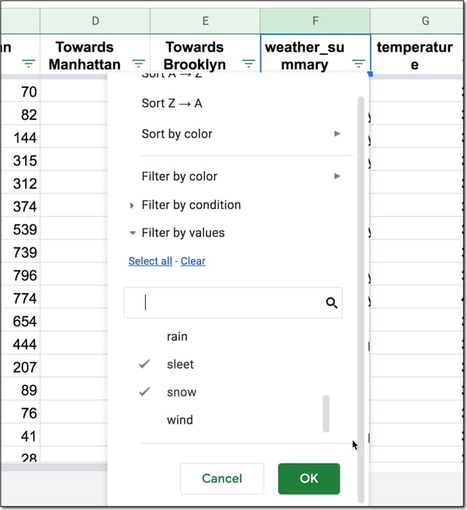
Click on the filter on the weather_summary column to open the filter menu.
Click “Clear” to deselect all the items.
Then choose “sleet” and “snow” as your filter values.
Hit OK to implement the filter.
You end up with 61 rows of data showing only the “sleet” or “snow” rows.
Now let’s see that same filter in BigQuery.
Step 12: WHERE filter keyword
Add the WHERE clause after the FROM line, and use the OR statement to filter on two conditions.
SELECT
  *
FROM
  `start-bigquery-294922.start_bigquery.brooklyn_bridge_pedestrians`
WHERE
  weather_summary = 'snow' OR weather_summary = 'sleet'
Check the count of the rows outputted by the this query. It’s 61, which matches the row count from your Google Sheet.
Ordering Data
Another common operation we want to do to understand our data is sort it. In Sheets we can either sort through the filter menu options or through the Data menu.
Step 13: Sorting data in Google Sheets
Remove the sleet and snow filter you applied above.
On the temperature column, click the Sort A → Z option, to sort the lowest temperature records to the top.
(Quick aside: it’s amazing to still see so many people walking across the bridge in sub-zero temps!)
Let’s recreate this sort in BigQuery.
Step 14: ORDER BY sort keyword
Add the ORDER BY clause to your query, after the FROM clause:
SELECT
  *
FROM
  `start-bigquery-294922.start_bigquery.brooklyn_bridge_pedestrians`
ORDER BY
  temperature ASC;
Use the keyword ASC to sort ascending (A – Z) or the keyword DESC to sort descending (Z – A).
You might notice that the first two records that show up have “null” in the temperature column, which means that no temperature value was recorded for those rows or it’s missing.
Let’s filter them out with the WHERE clause, so you can see how the WHERE and ORDER BY fit together.
Step 15: Filter out null values
The WHERE clause comes after the FROM clause but before the ORDER BY.
Remove the nulls by using the keyword phrase “IS NOT NULL”.
SELECT
  *
FROM
  `start-bigquery-294922.start_bigquery.brooklyn_bridge_pedestrians`
WHERE
  temperature IS NOT NULL
ORDER BY
  temperature ASC;
Aggregating Data
In Google Sheets, we group data with a pivot table.
Typically you choose a category for the rows and aggregate (summarize) the data into each category.
In this dataset, we have a row of data for each hour of each day. We want to group all 24 rows into a single summary row for each day.
Step 16: Pivot tables in Google Sheets
With your cursor somewhere in the pedestrian dataset, click Data < Pivot table
In the pivot table, add hour_beginning to the Rows.
Uncheck the “Show totals” checkbox.
Right click on one of the dates in the pivot table and choose “Create pivot date group“.
Select “Day of the month” from the list of options.
Add hour_beginning to Rows again, and move it so it’s the top category in Rows.
Check the “Repeat row labels” checkbox.
Right click on one of the dates in the pivot table and choose “Year-Month” from the list of options.
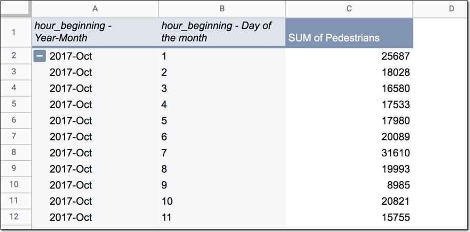
Add Pedestrians field to the Values section, and leave it set to the default SUM.
Your pivot table should look like this, with the total pedestrian counts for each day:
Now let’s recreate this in BigQuery.
If you’ve ever used the QUERY function in Google Sheets then you’re probably familiar with the GROUP BY keyword. It does exactly what the pivot table in Sheets does and “rolls up” the data into the summary categories.
Step 17: GROUP BY in BigQuery to aggregate data
First off, you need to use the EXTRACT function to extract the date from the timestamp in BigQuery.
This query selects the extracted date and the original timestamp, so you can see them side-by-side:
SELECT
  EXTRACT(DATE FROM hour_beginning) AS bb_date,
  hour_beginning
FROM
  `start-bigquery-294922.start_bigquery.brooklyn_bridge_pedestrians`
The EXTRACT DATE function turns “2017-10-01 00:00:00 UTC” into “2017-10-01”, which lets us aggregate by the date.
Modify the query above to add the SUM(Pedestrians) column, remove the “hour_beginning” column you no longer need and add the GROUP BY clause, referencing the grouping column by the alias name you gave it “bb_date”
SELECT
  EXTRACT(DATE FROM hour_beginning) AS bb_date,
  SUM(Pedestrians) AS bb_pedestrians
FROM
  `start-bigquery-294922.start_bigquery.brooklyn_bridge_pedestrians`
GROUP BY
  bb_date
The output of this query will be a table that matches the data in your pivot table in Google Sheet. Great work!
Functions in BigQuery
You’ll notice we used a special function (EXTRACT) in that previous query.
Like Google Sheets, BigQuery has a huge library of built-in functions. As you make progress on your BigQuery journey, you’ll find more and more of these functions to use.
For more information on functions in BigQuery, have a look at the function reference.
We saw the WHERE clause earlier, which lets you filter rows in your dataset.
However, if you aggregate your data with a GROUP BY clause and you want to filter this grouped data, you need to use the HAVING keyword.
Remember:
WHERE = filter original rows of data in dataset
HAVING = filter aggregated data after a GROUP BY operation
To conceptualize this, let’s apply the filter to our aggregate data in the Google Sheet pivot table.
Step 18: Pivot table filter in Google Sheets
Add hour_beginning to the filter section of your pivot table in Google Sheets.
Filter by condition and set it to Date is before > exact date > 11/01/2017
This filter removes rows of data in your Pivot Table where the data is on or after 1 November 2017. It leaves just the October 2017 data.
By now, I think you know what’s coming next.
Let’s apply that same filter condition in BigQuery using the HAVING keyword.
Step 19: HAVING filter keyword
Add the HAVING clause to your existing query, to filter out data on or after 1 November 2017.
Only data that satisfies the HAVING condition (less than 2017-11-01) is included.
SELECT
  EXTRACT(DATE FROM hour_beginning) AS bb_date,
  SUM(Pedestrians) AS bb_pedestrians
FROM
  `start-bigquery-294922.start_bigquery.brooklyn_bridge_pedestrians`
GROUP BY
  bb_date
HAVING
  bb_date < '2017-11-01'
The output of this query is 31 rows of data, for each day of the month of October.
Get started with Google BigQuery: Joining Data
A SQL Query walks into a bar.
In one corner of the bar are two tables.
The Query walks up to the tables and asks:
Mind if I join you?
JOIN pulls multiple tables together, like the VLOOKUP function in Google Sheets. Let's start in your Google Sheet.
Step 20: Vlookup to join data tables in Google Sheets
Create a new blank Sheet inside your Google Sheet.
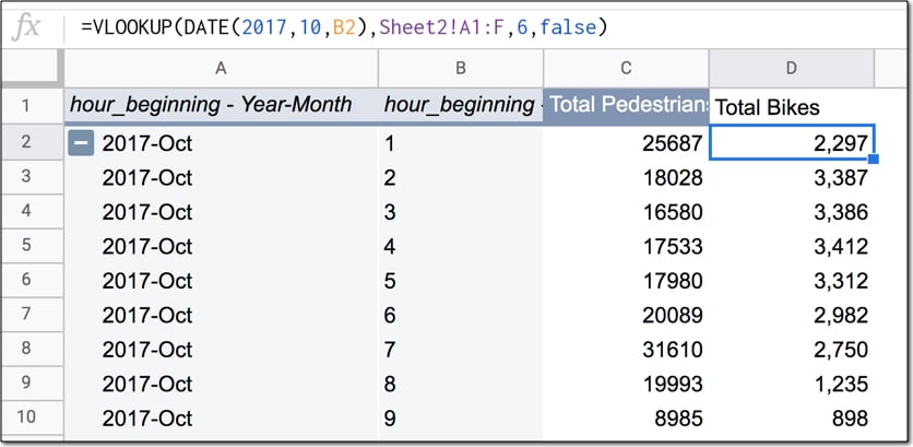
Drag the formula down the rows to complete the dataset.
The data in your Sheet now looks like this:
That's great!
We summarized the pedestrian data by day and joined the bicycle data to it, so you can compare the two numbers.
As you can see, there's around 10k - 20k pedestrian crossings/day and about 2k - 3k bike crossings/day.
Joining tables in BigQuery
Let's recreate this table in BigQuery, using a JOIN.
Step 21: Upload bicycle data to BigQuery
Following step 5 above, create a new table in your start_bigquery dataset and upload the second dataset, of bike data for NYC bridges from October 2017.
Name your table "nyc_bridges_bikes"
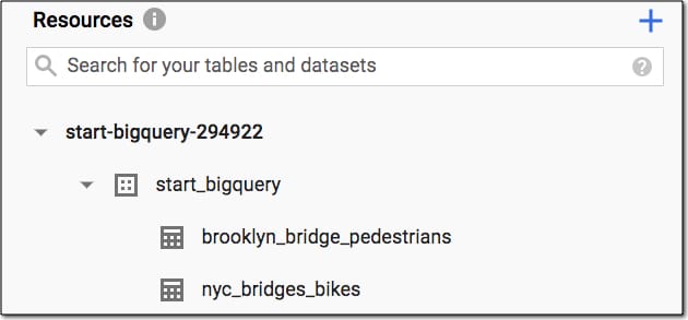
Your project should now look like this in the Resources pane in the left sidebar:
What we want to do now is take the table the you created above, with pedestrian data per day, and add the bike counts for each day to it.
To do that we use an INNER JOIN.
There are several different types of JOIN available in SQL, but we'll only look at the INNER JOIN in this article. It creates a new table with only the rows from each of the constituent tables that meet the join condition.
In our case the join condition is matching dates from the pedestrian table and the bike table.
We'll end up with a table consisting of the date, the pedestrian data and the bike data.
Ready? Let's go.
Step 22: JOIN the datasets in BigQuery
First, wrap the query you wrote above with the WITH clause, so you can refer to the temporary table that's created by the name "pedestrian_table".
WITH pedestrian_table AS (
  SELECT
    EXTRACT(DATE FROM hour_beginning) AS bb_date,
    SUM(Pedestrians) AS bb_pedestrians
  FROM
    `start-bigquery-294922.start_bigquery.brooklyn_bridge_pedestrians`
  GROUP BY
    bb_date
  HAVING
    bb_date < '2017-11-01'
)
Next, select both columns from the pedestrian table and one column from the bike table:
SELECT
  pedestrian_table.bb_date,
  pedestrian_table.bb_pedestrians,
  bike_table.Brooklyn_Bridge AS bb_bikes
FROM
  pedestrian_table
Of course, you need to add in the bike table to the query so the bike data can be retrieved:
INNER JOIN
  `start-bigquery-294922.start_bigquery.nyc_bridges_bikes` AS bike_table
Finally, specify the join condition, which tells the query what columns to match:
ON
  pedestrian_table.bb_date = bike_table.Date
Phew, that's a lot!
Here's the full query:
WITH pedestrian_table AS (
  SELECT
    EXTRACT(DATE FROM hour_beginning) AS bb_date,
    SUM(Pedestrians) AS bb_pedestrians
  FROM
    `start-bigquery-294922.start_bigquery.brooklyn_bridge_pedestrians`
  GROUP BY
    bb_date
  HAVING
    bb_date < '2017-11-01'
)
SELECT
  pedestrian_table.bb_date,
  pedestrian_table.bb_pedestrians,
  bike_table.Brooklyn_Bridge AS bb_bikes
FROM
  pedestrian_table
INNER JOIN
  `start-bigquery-294922.start_bigquery.nyc_bridges_bikes` AS bike_table
ON
  pedestrian_table.bb_date = bike_table.Date
You'll notice that the names of the columns in our SELECT clause are preceded by the table name, e.g. "pedestrian_table.bb_date".
This ensures there is no confusion over which columns from which tables are being requested. It’s also necessary when you join tables that have common column headings.
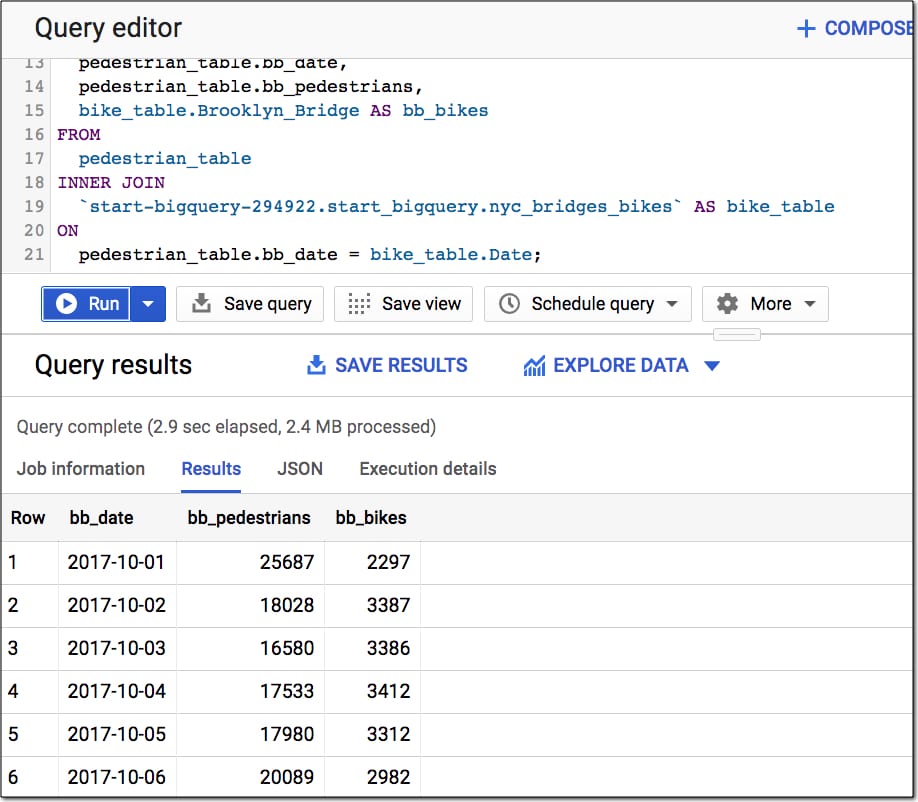
The output of this query is the same as the table you created in your Google Sheet step 20 (using the pivot table and VLOOKUP).
Formatting Your Queries
Last couple of things to mention with the SQL syntax is how to add comments and format your queries.
Step 23: Formatting Your Queries
You can add comments in SQL two ways, with a double dash "--" or forward slash and star combination "/*...*/".
-- single line comment, ignored when the program is run
or
/* multi-line comment
everything between the slash-stars
is ignored by the program when it's run */
It's also a good habit to put SQL keywords on separate lines, to make it more readable.
Use the menu More > Format to do this automatically.
Section 5: Export Data Out Of BigQuery
You have a few options to export data out of BigQuery.
In the Query results section of the editor, click on the "SAVE RESULTS" button to:
Save as a CSV file
Save as a JSON file
Export query results to Google Sheets (up to 16,000 rows)
Copy to Clipboard
In this tutorial, we're going to export the data out of BigQuery and back into a Google Sheet, to create a chart. We're able to do this because the summary dataset we've created is small (it's aggregated data we want to use to create a chart, not the row-by-row data).
Explore BigQuery Data in Sheets or Data Studio
If you want to create a chart based on hundreds of thousands or millions of rows of data, then you can explore the data in Google Sheets or Data Studio directly, without taking it out of BigQuery.
Click on the "EXPLORE DATA" option in the Query results section of the editor:
Explore in Google Sheets using Connected Sheets (Enterprise customers only)
Explore directly in Data Studio
Get started with Google BigQuery: Export to Google Sheets
In this tutorial, the output table is easily small enough to fit in Google Sheets, so let's export the data out of BigQuery and into Sheets.
There, we'll create chart a chart showing the pedestrian and bike traffic across the Brooklyn Bridge.
Step 24: Export Data Out Of BigQuery
Run your query from step 22 above, which outputs a table with date, pedestrian count and bike count.
Click on the "SAVE RESULTS" and select Google Sheets.
Hit Save.
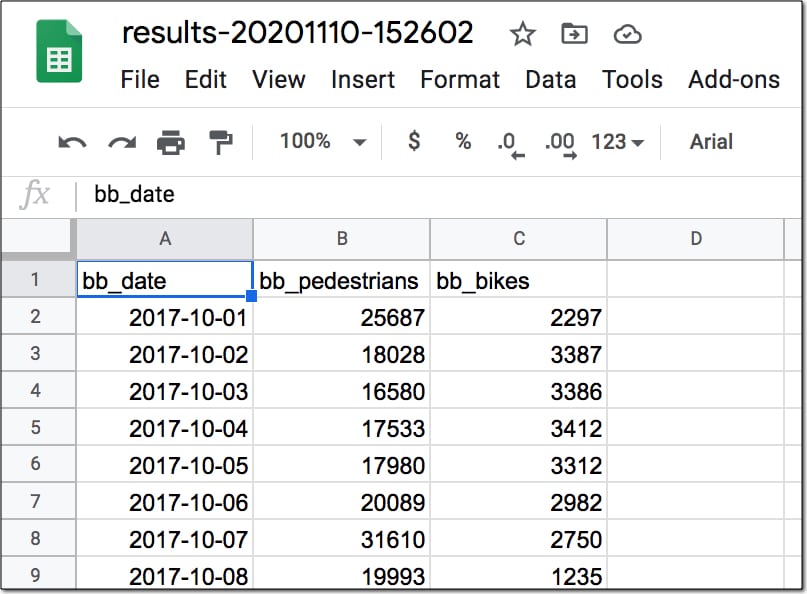
Select Open in the toast popup that tells you a new Sheet has been created, or find it in your Drive root folder (the top folder).
The data now looks like this in the new Sheet:
Yay! Back on familiar territory!
From here, you can do whatever you want with your data.
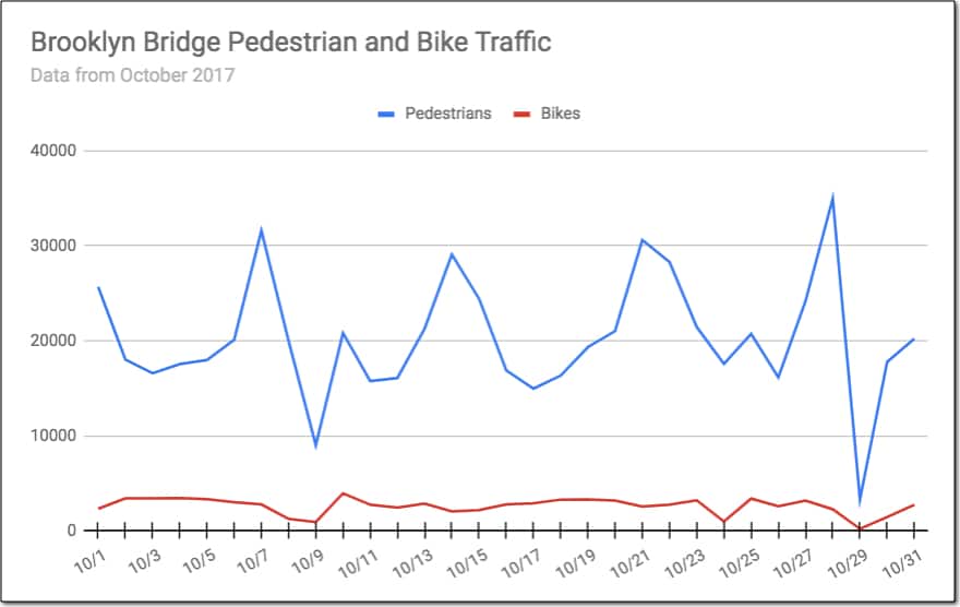
I chose to create a simple line chart to compare the daily foot and bike traffic across Brooklyn Bridge:
Step 25: Display the data in a chart in Google Sheets
Highlight your dataset and go to Insert > Chart
Select the line chart (if it isn't selected as the default).
Fix the title and change the column names to display better in chart.
Under the Horizontal Axis option, check the "Treat labels as text" checkbox.
See how much information this chart gives you, compared to thousands of rows of raw data.
It tells you the story of the pedestrian and bike traffic crossing the Brooklyn Bridge.
Congratulations!
You've completed your first end-to-end BigQuery + Google Sheets data analysis project.
Freezing rows and/or columns is a useful and simple technique to lock rows (or columns) of your spreadsheet so that they remain in view even as you scroll down your datasets. You’re anchoring them in place.
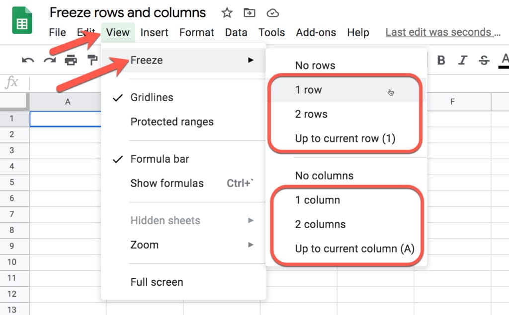
How To Freeze A Row In Google Sheets
Menu Method
Go to the menu: View > Freeze
Choose how many rows or columns you want to freeze: