In this post, you’ll learn how to find and highlight the top 5 values in Google Sheets.
For all the examples that follow, we’ll use this dataset, which is available in the downloadable template at the end of this post:
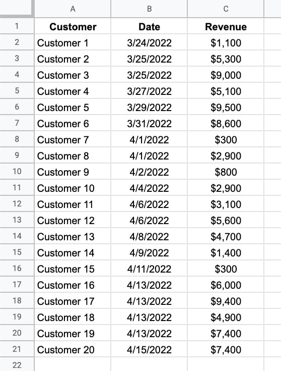
We’ll see how to highlight the rows with the top 5 values, as well as how to extract those values using SORTN.
Continue reading How To Highlight The Top 5 Values In Google Sheets With Formulas