Array Formulas have a fearsome reputation in the spreadsheet world (if you’ve even heard of them that is).
Array Formulas allow you to output a range of cells, rather than a single value. They also let you use non-array functions with arrays (think ranges) of data.
In this post I’m going to run through the basics of using array formulas, and you’ll see they’re really not that scary.
Hip, Hip Array!
What are array formulas in Google Sheets?
First of all, what are they?
To the uninitiated, they’re mysterious. Elusive. Difficult to understand. Yes, yes, and yes, but they are incredibly useful in the right situations.
Per the official definition, array formulas enable the display of values returned into multiple rows and/or columns and the use of non-array functions with arrays.
In a nutshell: whereas a normal formula outputs a single value, array formulas output a range of cells!
The easiest way to understand this is through an example.
Imagine we have this dataset, showing the quantity and item cost for four products:
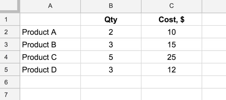
and we want to calculate the total cost of all four products.
We could easily do this by adding a formula in column D that multiplies B and C, and then add a sum at the bottom of column D.
However, array formulas let us skip that step and get straight to the answer with a single formula.
 💡 Learn more
Learn more about working with Advanced Formulas in the Advanced Formulas in Google Sheets course
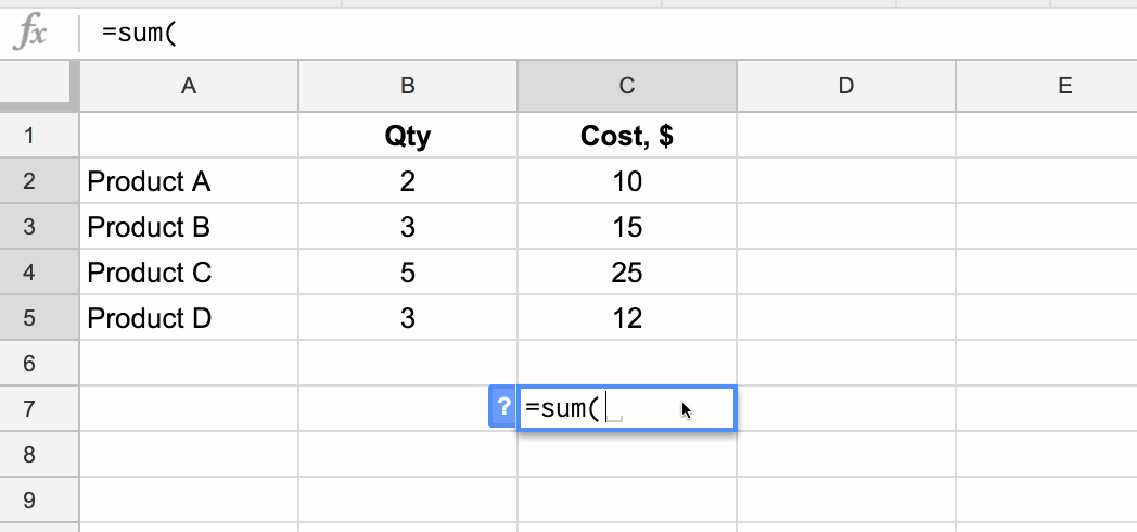
What’s the formula?
=ArrayFormula(SUM(B2:B5 * C2:C5))How does this formula work?
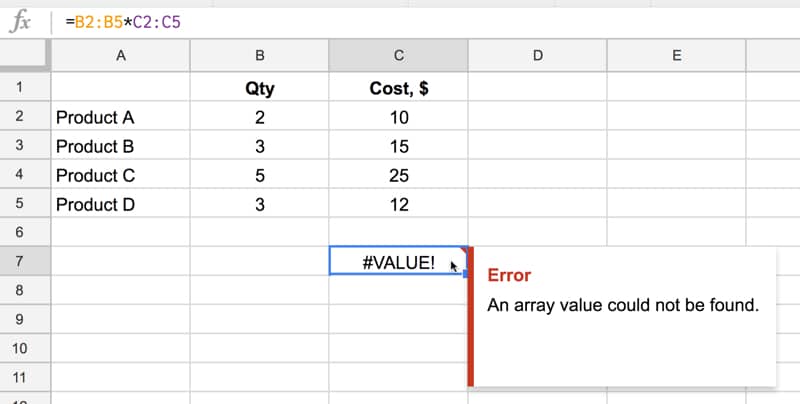
Ordinarily, when we use the multiplication (*) operator in a Sheet, we give it two numbers or two cells to multiply together.
However, in this case we’re giving it two ranges, or two arrays, of data:
= B2:B5 * C2:C5However, when we hit Enter this gives us a #VALUE! error as shown here:
We need to tell Google Sheets we want this to be an Array Formula. We do this in two ways.
Either type in the word ArrayFormula and add an opening/closing brackets to wrap your formula, or, more easily, just hit Ctrl + Shift + Enter (Cmd + Shift + Enter on a Mac) and Google Sheets will add the ArrayFormula wrapper for us.
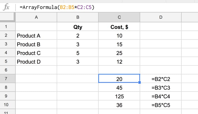
=ArrayFormula(B2:B5 * C2:C5)Now it works, and Google Sheets will output an array with each cell corresponding to a row in the original arrays, as shown in the following image:
Effectively what’s happening is that for each row, Google does the calculation and includes that result in our output array (here showing the equivalent formulas):
and another view, showing how the calculation is performed (just for the first and last row):
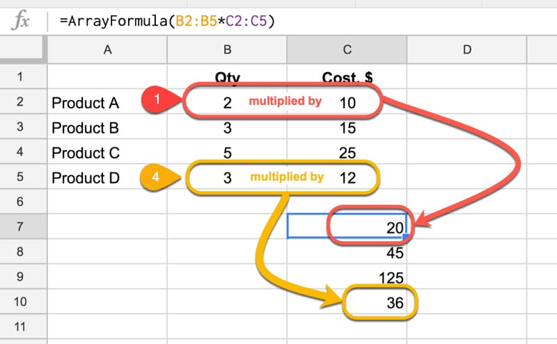
Note: array formulas only work if the size of the two arrays match, in this case each one has 4 numbers, so each row multiplication can happen.
Finally, we simply include the SUM function to add the four numbers:
=ArrayFormula(SUM(B2:B5 * C2:C5))as follows:
Quick Aside:
This calculation could also be done with the SUMPRODUCT formula, which takes array values as inputs, multiplies them and adds them together:
=SUMPRODUCT(B2:B5 , C2:C5)Another Array Formula Multiplication Example
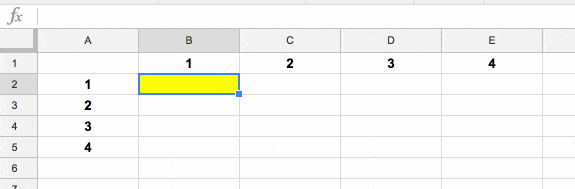
In this example, we enter a single formula to multiply an array of row headings against an array of column headings.
This only works because the dimensions of the arrays are compatible, since the number of columns in the first matrix is equal to the number of rows in the second matrix:
Array Formula With IF Function
This is an example of a non-array function being used with arrays (ranges). It works because we designate the IF formula as an Array Formula.
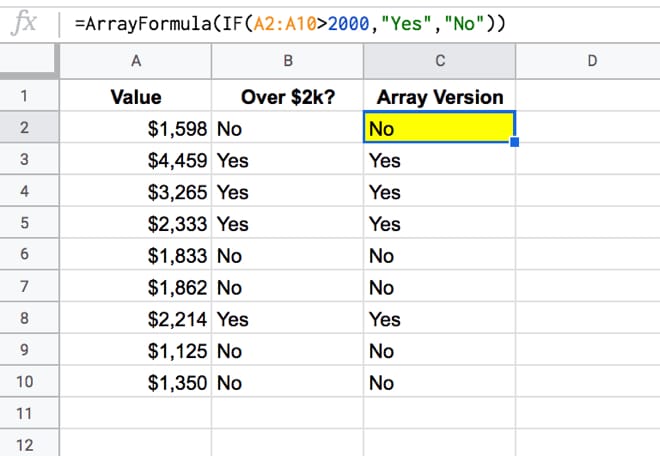
Consider a standard IF statement which checks whether a value in column A is over $2,000 or not:
=IF(A2>2000,"Yes","No")This formula would then be copied into each row where we want to run the test.
We can change this to a single Array Formula at the top of the column and run the IF statement across all the rows at once. For example, suppose we had values in rows 2 to 10 then we create a single Array Formula like this:
=ArrayFormula(IF(A2:A10>2000,"Yes","No"))This single formula, on row 2, will create an output array that fills rows 2 to 10 with “Yes”/”No” answers, as shown in the following image:
Can I see the example worksheet?
Click here to make your own copy
Related Articles
 Use Array Formulas With Google Forms Data
See how to use Array Formulas with Google Forms data to automatically calculate running metrics on your data, like sum, average, % of total and others.
 18 best practices for working with data in Google Sheets
This article describes 18 best practices for working with data in Google Sheets, including examples and screenshots to illustrate each concept.
 How to Remove Duplicates in Google Sheets
Learn how to remove duplicates in Google Sheets with these five different techniques, using Add-ons, Formulas, Formatting, Pivot Tables or Apps Script.