Unpivot in Google Sheets is a method to turn “wide” tables into “tall” tables, which are more convenient for analysis.
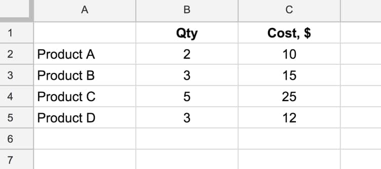
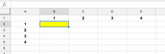
Suppose we have a wide table like this:
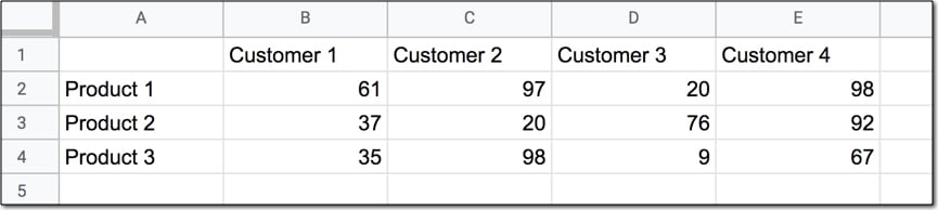
Wide data like this is good for the Google Sheets chart tool but it’s not ideal for creating pivot tables or doing analysis. The main reason is that data is captured in the column headings, which prevents you using it in pivot tables for analyis.
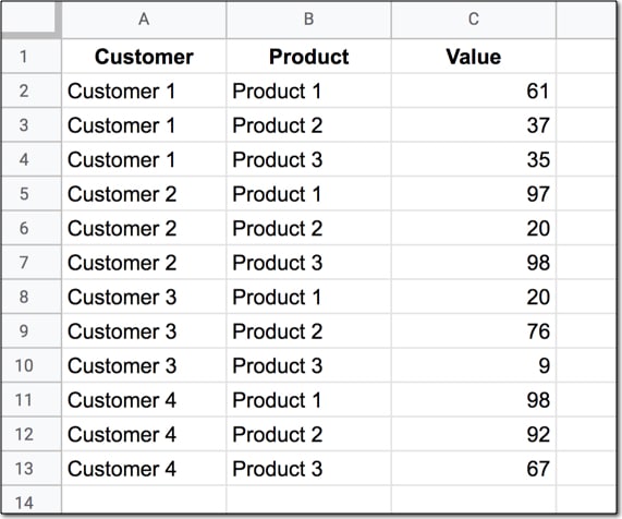
So we want to transform this data — unpivot it — into the tall format that is the way databases store data:
But how do we unpivot our data like that?
It turns out it’s quite hard.
It’s harder than going the other direction, turning tall data into wide data tables, which we can do with a pivot table.
This article looks at how to do it using formulas so if you’re ready for some complex formulas, let’s dive in…
Unpivot in Google Sheets
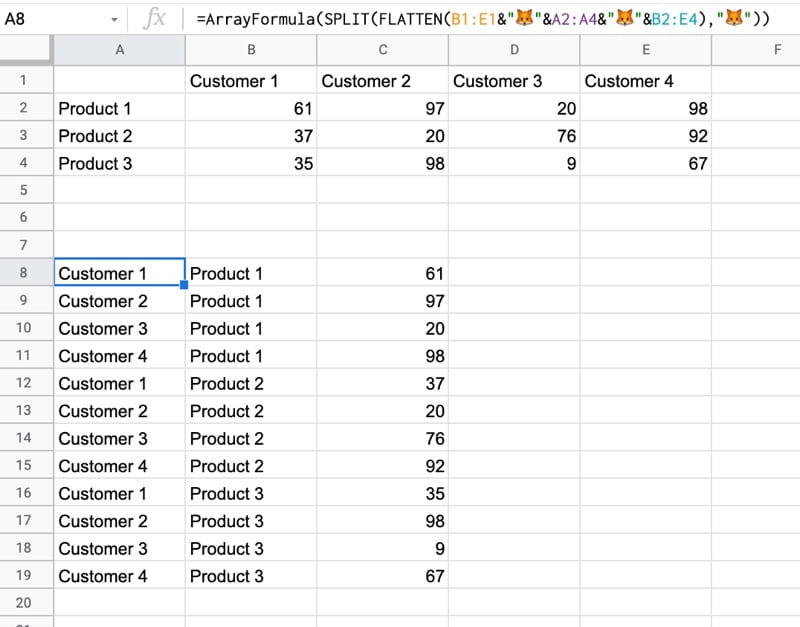
We’ll use the wide dataset shown in the first image at the top of this post.
The output of our formulas should look like the second image in this post.
In other words, we need to create 16 rows to account for the different pairings of Customer and Product, e.g. Customer 1 + Product 1, Customer 1 + Product 2, etc. all the way up to Customer 4 + Product 4.
Of course, we’ll employ the Onion Method to understand these formulas.
Template
Click here to open the Unpivot in Google Sheets template
Feel free to make your own copy (File > Make a copy…).
(If you can’t open the file, it’s likely because your G Suite account prohibits opening files from external sources. Talk to your G Suite administrator or try opening the file in an incognito browser.)
Step 1: Combine The Data
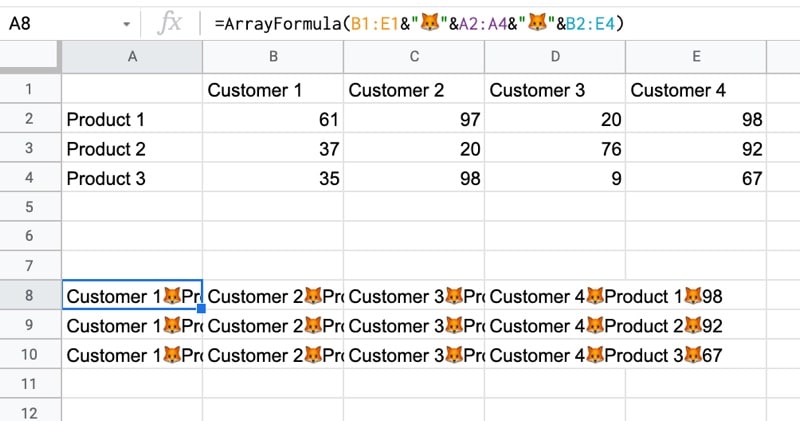
Use an array formula like this to combine the column headings (Customer 1, Customer 2, etc.) with the row headings (Product 1, Product 2, Product 3, etc.) and the data.
It’s crucial to add a special character between these sections of the dataset though, so we can split them up later on. I’ve used the fox emoji (because, why not?) but you can use whatever you like, provided it’s unique and doesn’t occur anywhere in the dataset.
=ArrayFormula(B1:E1&"🦊"&A2:A4&"🦊"&B2:E4)The output of this formula is:
Step 2: Flatten The Data
Before the introduction of the FLATTEN function, this step was much, much harder, involving lots of weird formulas.
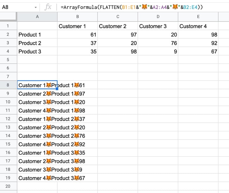
Thankfully the FLATTEN function does away with all of that and simply stacks all of the columns in the range on top of each other. So in this example, our combined data turns into a single column.
=ArrayFormula(FLATTEN(B1:E1&"🦊"&A2:A4&"🦊"&B2:E4))The result is:
Step 3: Split The Data Into Columns
The final step is to split this new tall column into separate columns for each data type. You can see now why we needed to include the fox emoji so that we have a unique character to split the data on.
Wrap the formula from step 2 with the SPLIT function and set the delimiter to “🦊”:
=ArrayFormula(SPLIT(FLATTEN(B1:E1&"🦊"&A2:A4&"🦊"&B2:E4),"🦊"))This splits the data into the tall data format we want. All that’s left is to add the correct column headings.
Unpivot With Apps Script
You can also use Google Apps Script to unpivot data, as shown in this example from the first answer of this Stack Overflow post.
Further Reading
For more information on the shape of datasets, have a read of Spreadsheet Thinking vs. Database Thinking.