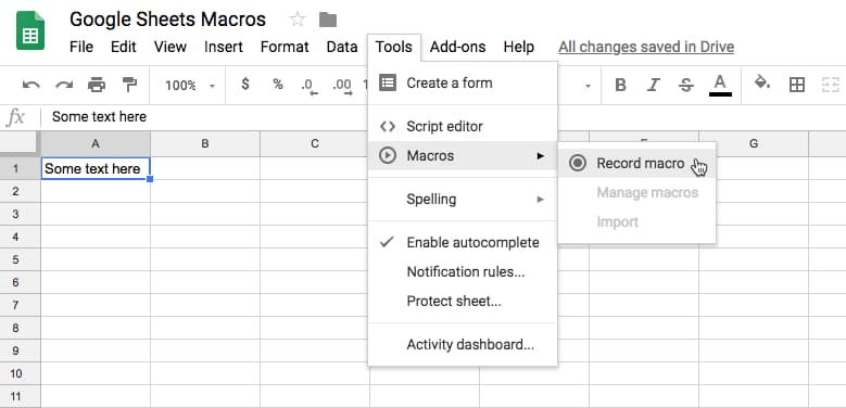
[Editor’s Note 2024: unfortunately, most of these solutions, which are 4+ years old, no longer work. Modern websites are built dynamically in the browser with JavaScript, and Google Sheets IMPORT functions no longer work in this case. If you’re still looking for reliable formula-style importing capabilities, check out the third-party tool IMPORTFROMWEB.
I’m leaving this article here for reference purposes as it shows interesting examples of XPath constructions.]
Google Sheets has a powerful and versatile set of IMPORT formulas that can import social media statistics.
This article looks at importing social media statistics from popular social media channels into a Google sheet, for social network analysis or social media management. If you manage a lot of different channels then you could use these techniques to set up a master view (dashboard) to display all your metrics in one place.
Contents
- Facebook
- Twitter
- Instagram
- Youtube
- Pinterest
- Alexa rank
- Quora
- Reddit
- Spotify
- Soundcloud
- GTmetrix
- Bitly
- Linkedin
- Sites that don’t work and why not
- Closing thoughts
- Resources
How to import social media statistics into Google Sheets with formulas
The formulas below are generally set up to return the number of followers (or page likes) for a given channel, but you could adapt them to return other metrics (such as follows) with a little extra work.
Caveats: these formulas occasionally stop working when the underlying website changes, but I will try to keep this post updated with working versions for the major social media statistics.
Example workbooks: Each example has a link to an associated Google Sheet workbook, so feel free to make your own copy: File > Make a copy....
 Import Facebook data
November 2018 update: The Facebook formula is working again! The trick is to use the mobile URL 😉 Thanks to reader Mark O. for this discovery.
Start with the mobile Facebook page URL in cell A1, e.g. this url
https://mobile.facebook.com/benlcollinsData
or this variation of it:
https://m.facebook.com/benlcollinsData
Here is the Google Sheets REGEX formula to extract page likes:
=INDEX(REGEXEXTRACT(REGEXEXTRACT(LOWER(INDEX(IMPORTXML(A1,"//@content"),2)),"([0-9km,.]+)(?: likes)"),"([0-9,.]+)([km]?)"),,1) * SWITCH(INDEX(REGEXEXTRACT(REGEXEXTRACT(LOWER(INDEX(IMPORTXML(A1,"//@content"),2)),"([0-9km,.]+)(?: likes)"),"([0-9,.]+)([km]?)"),,2),"k",1000,"m",1000000,1)
The following screenshot shows these formulas:
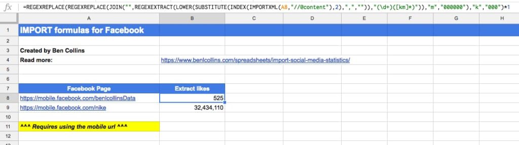
See the Facebook Import Sheet.
^ Back to Contents
 Import Twitter data
This formula is no longer working for extracting Twitter followers and I have not found an alternative.
Start with the mobile Twitter handle URL in cell A1, e.g.
https://mobile.twitter.com/benlcollins
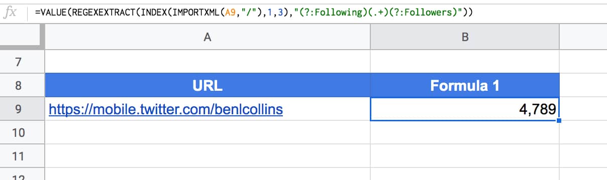
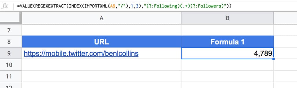
Here is the formula to extract follower count:
=VALUE(REGEXEXTRACT(IMPORTXML(A1,"/"),"(?:Following )([\d,]+)(?: Followers)"))
The following screenshot shows this formula:
Note 1: This Twitter formula seems to be particularly volatile, working fine one minute, then not at all the next. I have two Sheets open where it’ll work in one, but not the other!
See the Twitter Import Sheet.
^ Back to Contents
 Import Instagram data
This formula is no longer working for extracting Instagram followers and I have not found an alternative.
Start with the Instagram page URL in cell A1:
https://www.instagram.com/benlcollins/
Then, this formula in cell B1 to extract the follower metadata (this may or may not work):
=IMPORTXML(A1,"//meta[@name='description']/@content")
This extracts the following info: “230 Followers, 259 Following, 465 Posts – See Instagram photos and videos from Ben Collins (@benlcollins)”
Next step is to combine this with REGEX to extract the followers for example. Here’s the formula to do that (still assuming url in cell A1):
=INDEX(REGEXEXTRACT(REGEXEXTRACT(LOWER(IMPORTXML(A1,"//meta[@name='description']/@content")),"([0-9km,.]+)( followers)"),"([0-9,.]+)([km]?)"),,1) * SWITCH(INDEX(REGEXEXTRACT(REGEXEXTRACT(LOWER(IMPORTXML(A1,"//meta[@name='description']/@content")),"([0-9km,.]+)( followers)"),"([0-9,.]+)([km]?)"),,2),"k",1000,"m",1000000,1)
This deals with any accounts that have abbreviated thousands (k) or millions (m) notations.
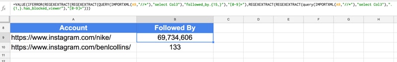
Alternative Approach
The following formulas to extract account metrics appear to only work for the instagram account when you are logged in. It makes use of the QUERY function, SPLIT function and INDEX function to do data wrangling inside the formula.
Here’s the number of followers:
=REGEXEXTRACT(INDEX(SPLIT(QUERY(IMPORTDATA(A1),"select Col1 limit 1 offset 181"),""""),1,2),"[\d,]+")
Here’s the number following:
=REGEXEXTRACT(QUERY(IMPORTDATA(A1),"select Col2 limit 1 offset 181"),"[\d,]+")
Here’s the number of posts:
=REGEXEXTRACT(QUERY(IMPORTDATA(A1),"select Col3 limit 1 offset 181"),"[\d,]+")
The following screenshot shows these formulas:
See the Instagram Import Sheet.
^ Back to Contents
 Import YouTube data
Start with the YouTube channel URL in cell A1:
https://www.youtube.com/benlcollins
To get the number of subscribers to a YouTube channel, use this formula in cell B1:
=VALUE(INDEX(REGEXEXTRACT(LOWER(INDEX(REGEXEXTRACT(INDEX(IMPORTXML(A1,"//div[@class='primary-header-actions']"),1,1),"(Unsubscribe)([0-9kmKM.]+)"),1,2)),"([0-9,.]+)([km]?)"),,1) * SWITCH(INDEX(REGEXEXTRACT(LOWER(INDEX(REGEXEXTRACT(INDEX(IMPORTXML(A1,"//div[@class='primary-header-actions']"),1,1),"(Unsubscribe)([0-9kmKM.]+)"),1,2)),"([0-9,.]+)([km]?)"),,2),"k",1000,"m",1000000,1))
See the YouTube Import Sheet.
^ Back to Contents
 Import Pinterest data
In cell A1, enter the following URL, again replacing benlcollins with the profile you’re interested in:
https://www.pinterest.com/bencollins/
Then in the adjacent cell, B1, enter the following formula:
=IMPORTXML(A1,"//meta[@property='pinterestapp:followers']/@content")
to get the following output (screenshot shows older version of the formula, latest one is above and in the template file):
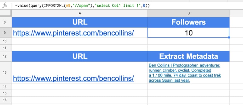
Note, you can also get hold of the profile metadata with the import formulas, as follows:
=IMPORTXML(A1,"//meta[@name='description']/@content")
See the Pinterest Import Sheet.
^ Back to Contents
 Import Alexa ranking data
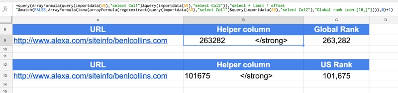
Here there are two metrics I’m interested in – a site’s Global rank and a site’s US rank.
Global Rank
To get the Global rank for your site, enter your URL into cell A1 (replace benlcollins.com):
http://www.alexa.com/siteinfo/benlcollins.com/
and use the following helper formula in cell B1:
=QUERY(ArrayFormula(QUERY(IMPORTDATA(A1),"select Col1") & QUERY(IMPORTDATA(A1),"select Col2")),"select * limit 1 offset " & MATCH(FALSE,ArrayFormula(ISNA(REGEXEXTRACT(QUERY(IMPORTDATA(A1),"select Col1") & QUERY(IMPORTDATA(A1),"select Col2"),"Global rank icon.{10,}"))),0)+1)
and then extract the rank in cell C1:
=VALUE(REGEXEXTRACT(B1,"[\d]{3,}"))
US Rank
Assuming you have the Alexa URL in cell A1 again, then the US rank is extracted with this helper formula:
=QUERY(ArrayFormula(QUERY(IMPORTDATA(A1),"select Col1") & QUERY(IMPORTDATA(A1),"select Col2")),"select * limit 1 offset " & MATCH(FALSE,ArrayFormula(ISNA(REGEXEXTRACT(QUERY(IMPORTDATA(A1),"select Col1") & QUERY(IMPORTDATA(A1),"select Col2"),"title='United States Flag'.alt.{50,}"))),0))
and this formula to extract the actual rank value:
=VALUE(REGEXEXTRACT(B1,"[\d]{3,}"))
The following screenshot shows these formulas:
See the Alexa Ranking Import Sheet.
^ Back to Contents
 Import Quora data
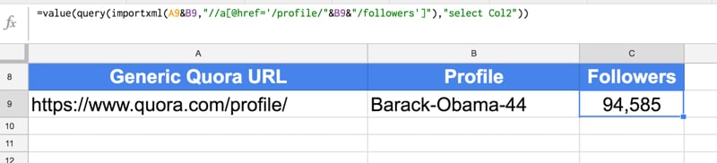
In this instance, I’ve imported the number followers Barack Obama has on Quora.
Quora is a little bit different because I need to use the URL and the profile name in my formula, so I’ve kept them in separate cells for that purpose. So in cell A1, add the generic Quora URL:
https://www.quora.com/profile/
And then in cell B1, add the profile name:
Barack-Obama-44
Then the formula in C1 to get the number of followers is:
=VALUE(QUERY(IMPORTXML(A1&B1,"//a[@href='/profile/"&B1&"/followers']"),"select Col2"))
The following screenshot shows this formula:
See the Quora Import Sheet.
^ Back to Contents
 Import Reddit data
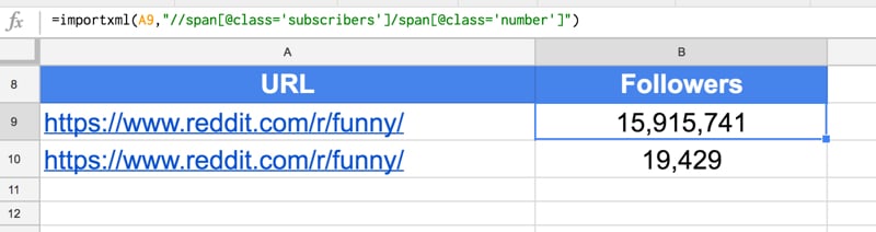
Here, I’m using the funny subreddit as my example.
In A1:
https://www.reddit.com/r/funny/
To get the number of followers of this subreddit, use this formula in cell B1:
=IMPORTXML(A1,"//span[@class='subscribers']/span[@class='number']")
Bonus: To get the number of active viewers of this subreddit:
=IMPORTXML(A1,"//p[@class='users-online']/span[@class='number']")
The following screenshot shows these formulas:
See the Reddit Import Sheet.
^ Back to Contents
 Import Spotify monthly listeners
Here’s a method for extracting the number of followers an artist has on the music streaming site Spotify.
First, find your favorite artist on Spotify: https://open.spotify.com/browse/featured
Copy the URL into cell A1 (it’ll look like this):
https://open.spotify.com/artist/2ye2Wgw4gimLv2eAKyk1NB
(This is Metallica, yeah ?)
Then put the following formula into cell A2 to extract the monthly listeners:
=N(INDEX(IMPORTXML(A1,"//h3"),2))
See the Spotify Import Sheet.
To get Spotify playlist data, add the playlist URL into cell A1:
https://open.spotify.com/playlist/37i9dQZF1DX1lVhptIYRda
And use this formula to extract the number of songs and likes:
=QUERY(SPLIT(REGEXEXTRACT(INDEX(IMPORTXML(A1,"//@content"),5),"^(?:[a-zA-Z. ]+ · Playlist · )([0-9]+ songs · [0-9.KM]+ likes)")," · "),"select Col1, Col3")
^ Back to Contents
 Import Soundcloud data
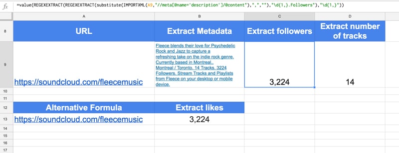
Start with the Soundcloud page URL in cell A1, e.g.
https://soundcloud.com/fleecemusic
Here is the formula to extract page likes:
=ArrayFormula(VALUE(REGEXEXTRACT(QUERY(SORT(IFERROR(REGEXEXTRACT( IMPORTXML(A1,"//script"),"followers_count..\d{1,}"),""),1,FALSE),"select * limit 1"),"\d{1,}")))
Alternative formula:
Here is an alternative formula to extract the page metadata, which includes the likes:
=IMPORTXML(A1,"//meta[@name='description']/@content")
the formula to extract likes is:
=VALUE(REGEXEXTRACT(REGEXEXTRACT(SUBSTITUTE( IMPORTXML(A1,"//meta[@name='description']/@content"),",",""),"\d{1,}.Followers"),"\d{1,}"))
and to extract the “talking about” number:
=VALUE(REGEXEXTRACT(REGEXEXTRACT(SUBSTITUTE( IMPORTXML(A1,"//meta[@name='description']/@content"),",",""),"\d{1,}.Tracks"),"\d{1,}"))
The following screenshot shows these formulas:
See the Soundcloud Import Sheet.
^ Back to Contents
 Import GTmetrix data
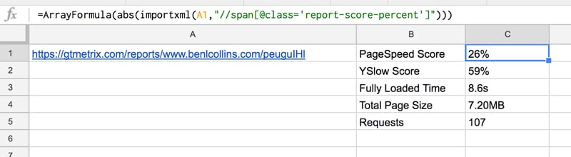
GTmetrix is a website that analyzes website performance.
You need to grab the correct URL before you can start scraping the data. So navigate to the GTmetrix site and enter the URL and hit analyze. You’ll end up with a URL like this:
https://gtmetrix.com/reports/www.benlcollins.com/BcHv78bP
Those last 8 characters (“BcHv78bP”) appear to be unique each time you run an analysis, so you’ll have to do this step manually.
Then in column B, I use this formula to extract the Page Speed Score and YSlow Score, into cells B1 and B2:
=ArrayFormula(ABS(IMPORTXML(A1,"//span[@class='report-score-percent']")))
and this formula in cell B3, to get the page details (Fully Loaded Time, Total Page Size and Requests) in cells B3, B4 and B5:
=IMPORTXML(A1,"//span[@class='report-page-detail-value']")
The following screenshot shows these formulas:
See the GTmetrix Import Sheet.
^ Back to Contents
 Import Bitly click data
Bitly is a service for shortening urls. They provide metrics for how many clicks you’ve had on each bitly link, e,g.
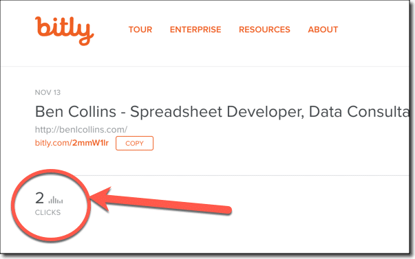
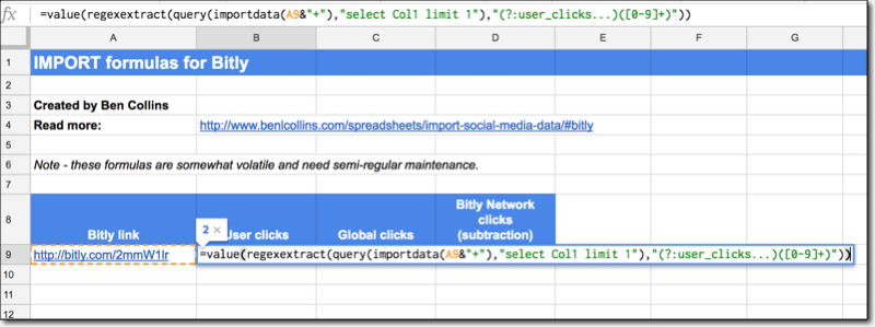
Taking a standard Bitly link (e.g. http://bitly.com/2mmW1lr) and appending a “+” to it will take you to the dashboard page, with the metrics. Then we can use the import data function, a query function and a REGEX function to extract the click metrics.
User clicks are:
=VALUE(REGEXEXTRACT(QUERY(IMPORTDATA(A9&"+"),"select Col1 limit 1"),"(?:user_clicks...)([0-9]+)"))
and global clicks are:
=VALUE(REGEXEXTRACT(QUERY(IMPORTDATA(A9&"+"),"select Col5"),"(?:global_clicks:.)([0-9]+)"))
Clicks from the Bitly network are then simply the user clicks subtracted from the global clicks.
The following screenshot shows these formulas:
See the Bitly Import Sheet.
^ Back to Contents
 Import Linkedin data
This formula is no longer working for extracting Linkedin followers and I have not found an alternative.
In cell A1:
https://www.linkedin.com/in/benlcollins/
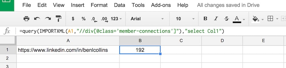
This formula used to work to get the number of Linkedin followers, but no longer:
=QUERY(IMPORTXML(A1,"//div[@class='member-connections']"),"select Col1")
and the output:
There is no example sheet for Linkedin since the formula is no longer working.
^ Back to Contents
 Sites that don’t work and why not
I’ve tried the following sites but the IMPORT formulas are unable to extract the social media statistics:
- Linkedin (see above)
- Similar Web
- Twitch
- Mobcrush
- Crunchbase
- Angel.co
- Majestic SEO
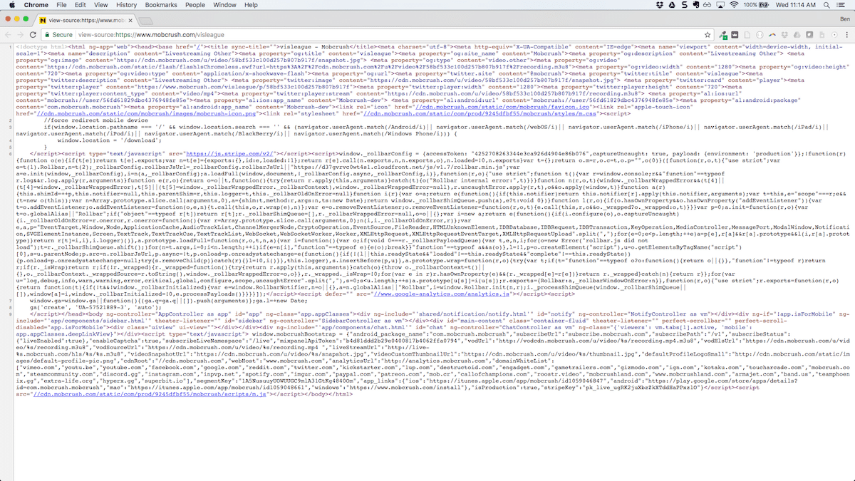
These are all modern sites built using front-end, client-side Javascript frameworks, so the IMPORT formulas can’t extract any data because the page is built dynamically in browser as it’s loaded up. The IMPORT formulas work fine on sites built in the traditional fashion, with lots of well formed HTML tags, where the social media statistics are embedded into the site markup that is passed from the server.
Compare this screenshot of the source code for Mobcrush, built using Angular JS it looks like (click to enlarge):
versus what the source code looks for this page on my website (click to enlarge):
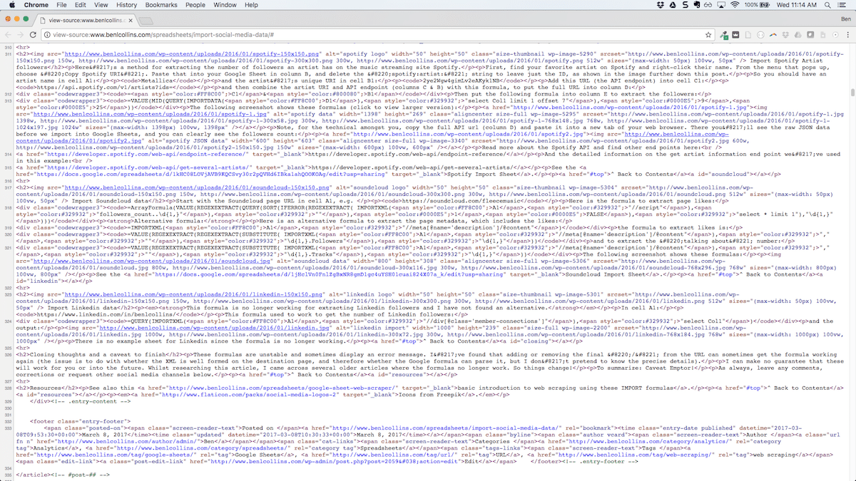
You can see the code for my site has lots of tags which the IMPORT formulas can parse, whereas the other site’s code does not.
If anyone knows of any clever way to get around this, do share!
Otherwise, you’re next option is to venture down the API route. Yes, this involves coding, but it’s not as hard as you think.
I’ll be posting some API focussed articles soon. In the meantime, check out my post on how to get started with APIs, or for a peak at what’s coming, take a look at my Apps Script + API repo on GitHub.
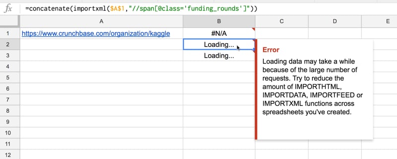
Loading error
Also, even when these formulas are working, they can be temperamental. If you work with them a lot, sooner or later you’ll find yourself hitting this loading issue all the time, where the formulas stop displaying any results:
^ Back to Contents
 Closing thoughts
These formulas are unstable and will sometimes display an error message.
I’ve found that adding or removing the final “/” from the URL can sometimes get the formula working again (the issue is to do with caching).
I can make no guarantee that these will work for you or into the future. Whilst researching this article, I came across several older articles where many of the formulas no longer work. So things change!
To summarize: Caveat Emptor!
^ Back to Contents
 Resources
^ Back to Contents
As always, leave any comments, corrections or request other social media statistics below.
Icons from Freepik.