Category: Spreadsheets

The IFS function in Google Sheets is used to test multiple conditions and outputs a value specified by the first test that evaluates to true.

It’s akin to a nested IF formula, although it’s not exactly the same. However, if you find yourself creating a nested IF formula then it’s probably easier to use this IFS function.

Continue reading IFS Function in Google Sheets

The SPLIT function in Google Sheets is used to divide a text string (or value) around a given delimiter, and output the separate pieces into their own cells.

SPLIT Function Examples

Let’s see a simple example using SPLIT to separate a list of names in cell A1:

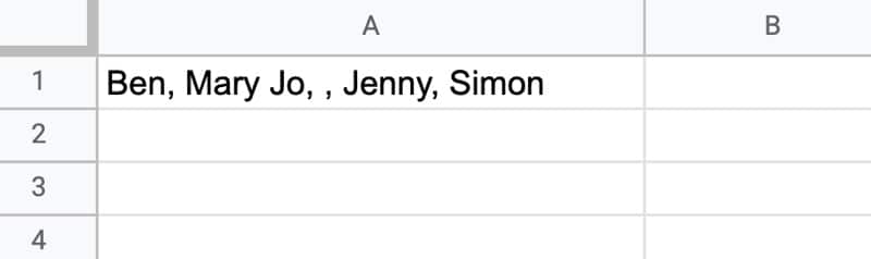
This simple SPLIT formula will separate these names, using the comma as the separator:

The result is 5 cells, each containing a name. Note that one cell looks blank because the text string in cell A1 has two adjacent commas with a space between them. The “space” is interpreted in the same way as the names and contained in the output:

Now watch what happens if we include a space in the delimiter, i.e. ", "

The function splits on the comma "," and on the space " ", so the name “Mary Jo” split in two:

This is probably not the desired behavior.

The third argument is an optional TRUE or FALSE that determines whether SPLIT considers each individual character of the delimiter (TRUE) or only the full combination as the separator to use (FALSE).

In our example, adding FALSE ensures that it only considers the combined comma/space string as the delimiter:

And the output looks like this:

There is a fourth argument too, which is optional and takes a TRUE/FALS value. It determines whether to remove blank cells or not in the output.

To illustrate this, consider this arrangement of data separated by semi-colons. Note the presence of two adjacent semi-colons with no data between them:

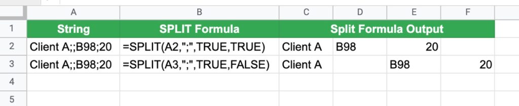
The fourth argument determines whether to show or hide the blank cell caused by the two adjacent semi-colons.

To keep the blank cells, add FALSE as the fourth argument:

SPLIT Function in Google Sheets: Syntax

It takes 4 arguments:

text

This is the text string or value in the cell that you want to split. It can also be a reference to a cell with a value in, or even the output of a nested formula, provided that output is a string or value and not an array.

delimiter

The character or characters used to split the text. Note that by default, all characters are used in the division. So a delimiter of “the” will split a text string on “the”, “he”,”t”,”h”,”e” etc.

This behavior can be controlled by the next argument:

split_by_each

This argument is optional and takes a TRUE or FALSE value only. If omitted, it’s assumed to be TRUE.

The TRUE behavior splits by individual characters in the delimiter and any combination of them. The FALSE behavior does not consider the characters separately, and only divides on the entire delimiter.

remove_empty_text

The fourth and final argument is optional and takes a TRUE or FALSE value only. If omitted, it’s assumed to be TRUE.

It specifies what to do with empty results in the SPLIT output. For example, suppose you’re splitting a text string with a "," and your string looks like this: “Ben,Bob,,Jenny,Anna”

Between the names Bob and Jenny are two commas with no value between them.

Setting this final argument of the SPLIT function to FALSE results in a blank cell in the output. If this fourth argument is omitted or set to TRUE, then the blank cell is removed and “Bob” and “Jenny” appear in adjacent cells.

SPLIT Function Notes

• Delimiters in SPLIT are case sensitive. So “t” only splits on lower-case t’s in the text
• The SPLIT function requires enough “space” for its output. If it splits a text string into 4 elements then it requires 4 cells (including the one the formula is in) on that row to expand into. If there is already data in any of these cells, it does NOT overwrite it but instead shows a #REF! error message
• You can input a range as the first argument to the SPLIT function, but it requires an Array Formula wrapper to work
• The output from the SPLIT function is an array of values that can be passed as the input into another formula, which may require the use of the Array Formula

Alternative Split Method

There’s an alternative way to split values in a Google Sheet.

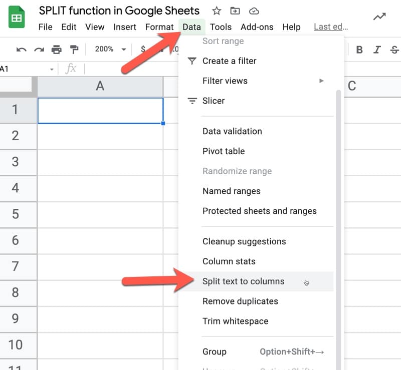
Under the Data menu, there’s a feature called “Split text to columns” which will separate single columns into multiple columns, based on the delimiter you specify.

It’s a quick and easy way to split text.

Note that it overwrites existing data in your Sheet if the split columns overlap with any existing data.

SPLIT Function Template

Click here to open a view-only copy >>

Feel free to make a copy: File > Make a copy…

If you can’t access the template, it might be because of your organization’s Google Workspace settings. If you click the link and open it in an Incognito window you’ll be able to see it.

You can also read about it in the Google documentation.

---

Advanced Examples of the SPLIT Formula in Google Sheets

Extract The N-th Word In A Sentence

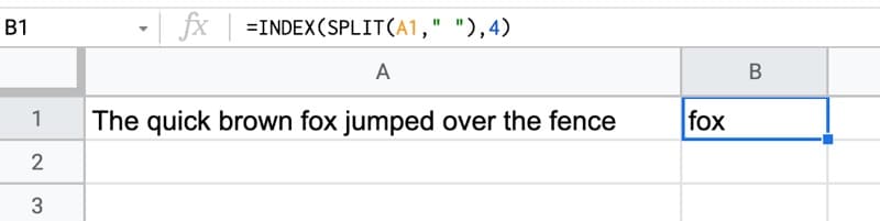
You can wrap the SPLIT function output with an INDEX function to extract the word at a given position in a sentence. E.g. to extract the 4th word, use this formula:

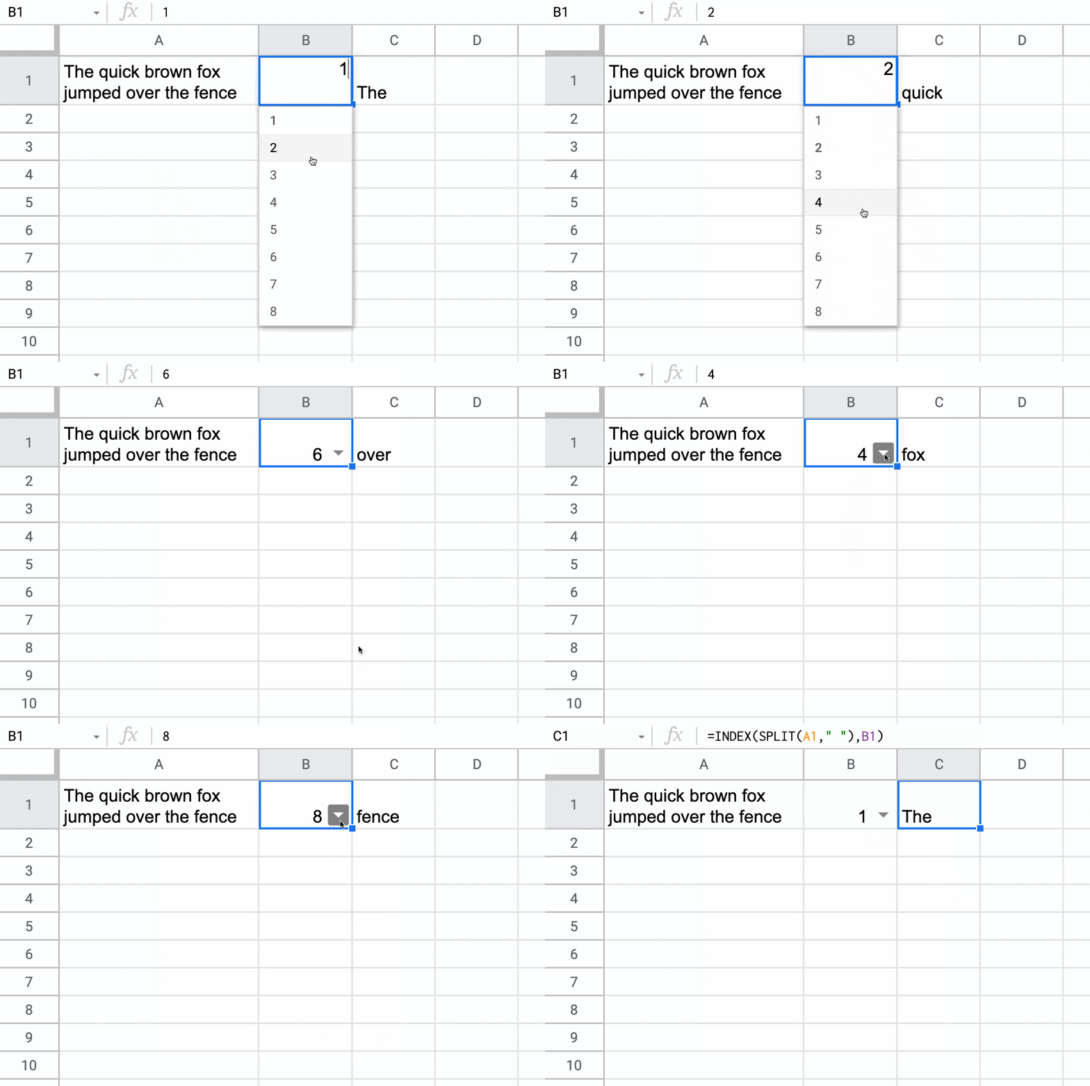
If you combine this with a drop down menu using data validation, you can create a word extractor:

Alphabetize Comma-Separated Strings With The SPLIT Function in Google Sheets

Suppose you have a list of words in a single cell that you want to sort alphabetically:

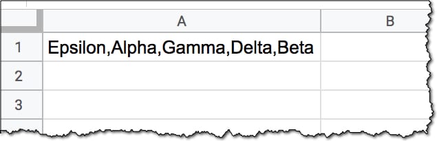
This formula will rearrange that list alphabetically:

It splits the string of words, applies the TRANSPOSE function to convert into a column so it can be sorted using the SORT function, and then recombines it with the JOIN function.

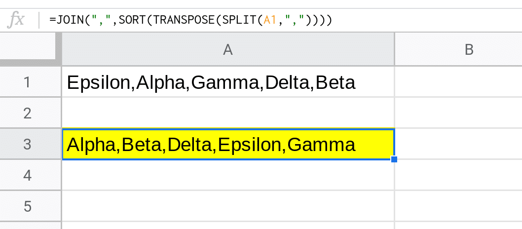
Read more in Formula Challenge #3: Alphabetize Comma-Separated Strings.

Splitting and Concatenating Strings

The SPLIT is useful in more advanced formulas as a way to divide an array into separate elements, do some work on those elements (e.g. sort them) before recombining them with another function, like the JOIN function.

For example, this array formula will add surnames to a list of first names in a cell:

which looks like this in your Google Sheet:

Using the onion framework to analyze this formula, starting from the innermost function and working out, it splits the text string, joins on the surname “Smith”, trims the excess trailing space with the TRIM function, and finally outputs an array by using the Array Formula.

Find Unique Items In A Grouped List

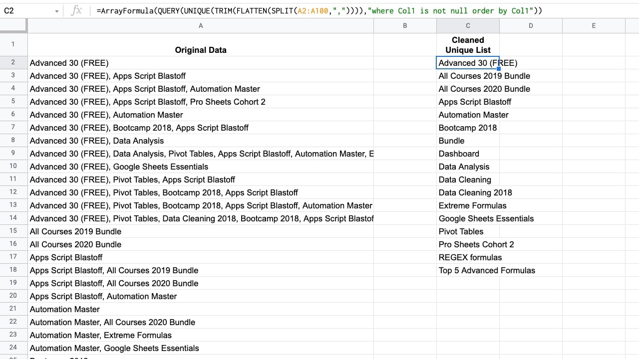
Suppose you want to find unique values from data that looks like this:

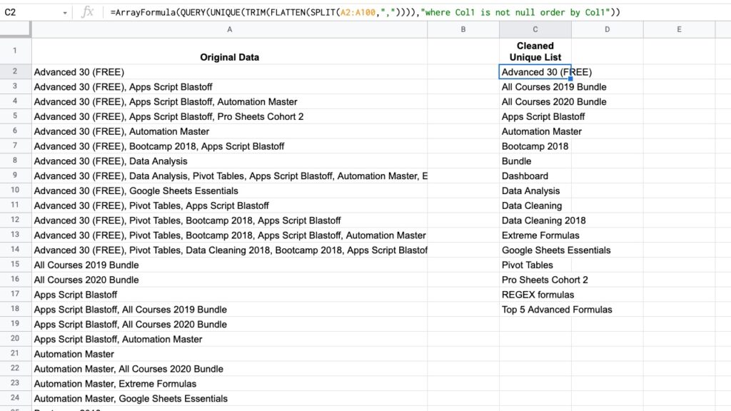
You want to extract a unique list of items from the column containing grouped words, which are separated by commas.

Use this formula to extract the unique values:

Read more about this technique in this post: Get A Unique List Of Items From A Column With Grouped Words

Unpivot Technique

The SPLIT function in Google Sheets is used in a number of the complex IMPORT formulas for retrieving social media statistics into your Google Sheet.

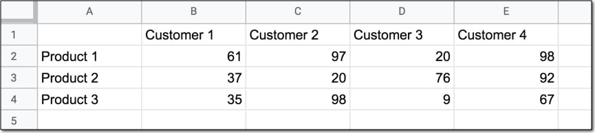
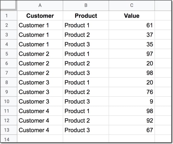
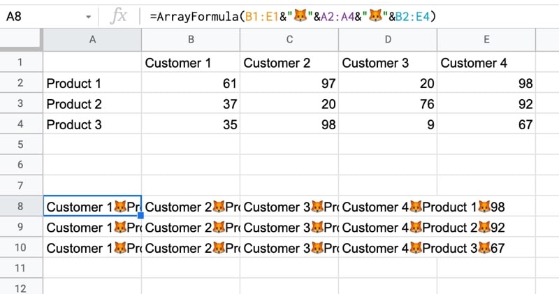
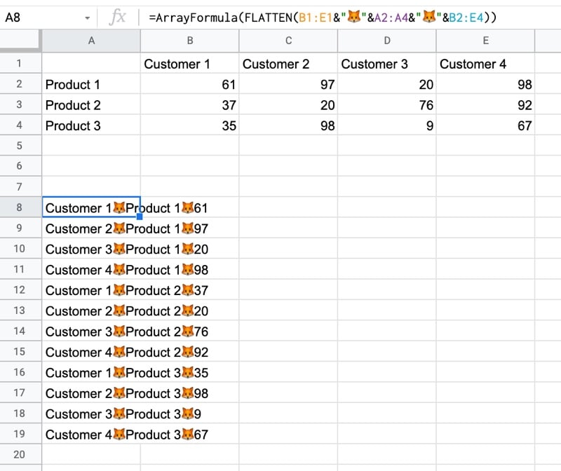
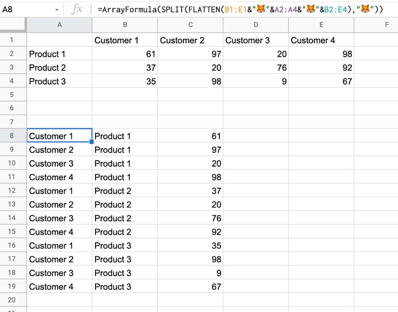
The SPLIT function was combined with the FLATTEN function in this exceedingly wacky unpivot formula in Google Sheets:

All in all, SPLIT is a useful function!

The REPT function in Google Sheets is used to repeat an expression a set number of times.

The REPT formula to repeat “Go! ” three times is:

Notice the additional space added after the exclamation point, so that there is a space between the repeated values in the output.

Continue reading REPT Function in Google Sheets