Unpivot In Google Sheets With Formulas (How To Turn Wide Data Into Tall Data)

Unpivot in Google Sheets is a method to turn “wide” tables into “tall” tables, which are more convenient for analysis.

Suppose we have a wide table like this:

Wide Data Table

Wide data like this is good for the Google Sheets chart tool but it’s not ideal for creating pivot tables or doing analysis. The main reason is that data is captured in the column headings, which prevents you using it in pivot tables for analyis.

So we want to transform this data — unpivot it — into the tall format that is the way databases store data:
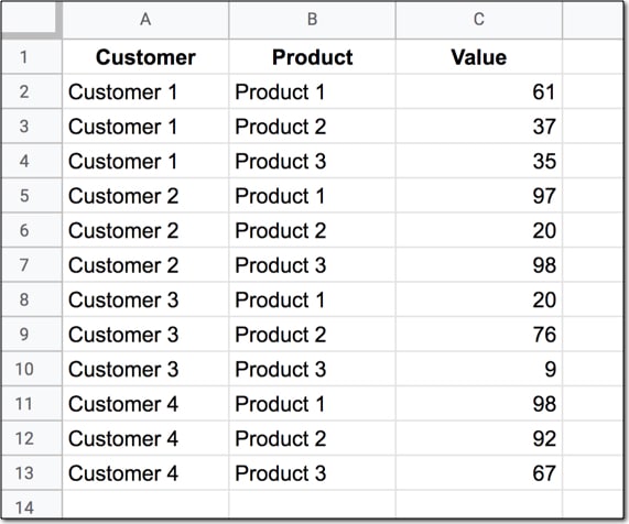
Unpviot in Google Sheets

But how do we unpivot our data like that?

It turns out it’s quite hard.

It’s harder than going the other direction, turning tall data into wide data tables, which we can do with a pivot table.

This article looks at how to do it using formulas so if you’re ready for some complex formulas, let’s dive in…

Unpivot in Google Sheets

We’ll use the wide dataset shown in the first image at the top of this post.

The output of our formulas should look like the second image in this post.

In other words, we need to create 16 rows to account for the different pairings of Customer and Product, e.g. Customer 1 + Product 1, Customer 1 + Product 2, etc. all the way up to Customer 4 + Product 4.

Of course, we’ll employ the Onion Method to understand these formulas.

Template

Click here to open the Unpivot in Google Sheets template

Feel free to make your own copy (File > Make a copy…).

(If you can’t open the file, it’s likely because your G Suite account prohibits opening files from external sources. Talk to your G Suite administrator or try opening the file in an incognito browser.)

Step 1: Combine The Data

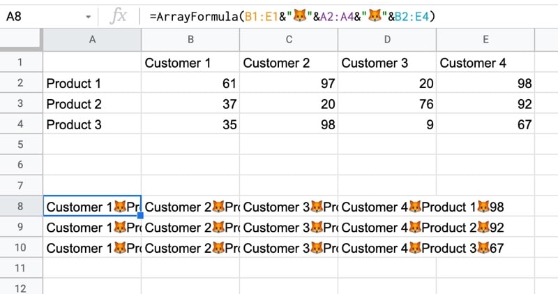
Use an array formula like this to combine the column headings (Customer 1, Customer 2, etc.) with the row headings (Product 1, Product 2, Product 3, etc.) and the data.

It’s crucial to add a special character between these sections of the dataset though, so we can split them up later on. I’ve used the fox emoji (because, why not?) but you can use whatever you like, provided it’s unique and doesn’t occur anywhere in the dataset.

=ArrayFormula(B1:E1&"🦊"&A2:A4&"🦊"&B2:E4)

The output of this formula is:

Unpivot Data In Google Sheets Step 1

Step 2: Flatten The Data

Before the introduction of the FLATTEN function, this step was much, much harder, involving lots of weird formulas.

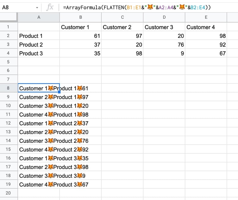
Thankfully the FLATTEN function does away with all of that and simply stacks all of the columns in the range on top of each other. So in this example, our combined data turns into a single column.

=ArrayFormula(FLATTEN(B1:E1&"🦊"&A2:A4&"🦊"&B2:E4))

The result is:

Unpivot Data In Google Sheets Step 2

Step 3: Split The Data Into Columns

The final step is to split this new tall column into separate columns for each data type. You can see now why we needed to include the fox emoji so that we have a unique character to split the data on.

Wrap the formula from step 2 with the SPLIT function and set the delimiter to “🦊”:

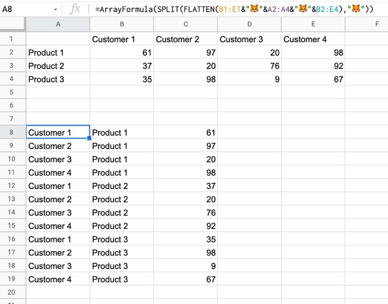
=ArrayFormula(SPLIT(FLATTEN(B1:E1&"🦊"&A2:A4&"🦊"&B2:E4),"🦊"))

This splits the data into the tall data format we want. All that’s left is to add the correct column headings.
Unpivot Data In Google Sheets Step 3

Unpivot With Apps Script

You can also use Google Apps Script to unpivot data, as shown in this example from the first answer of this Stack Overflow post.

Further Reading

For more information on the shape of datasets, have a read of Spreadsheet Thinking vs. Database Thinking.
Formula Challenge #5: Merge Columns in Google Sheets With Single Range Reference

This Formula Challenge originally appeared as Tip #131 of my weekly Google Sheets Tips newsletter, on 21 December 2020.

Sign up here so you don’t miss out on future Formula Challenges:


Find all the Formula Challenges archived here.

The Challenge: Merge Columns With Single Range Reference

Question: How can you merge n number of columns and get the unique values, without typing each one out?

In other words, can you create a single formula that gives the same output as this one:

=SORT( UNIQUE( {A:A;B:B;C:C;...;XX:XX} ))

but without having to write out A:A, B:B, C:C, D:D etc. and instead just write A:XX as in the input?

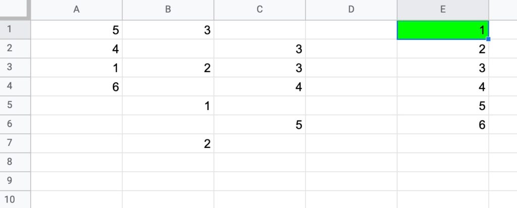
Use this simple dataset example, where your formula will be in cell E1 (in green):

Formula challenge 5 Data

Your answer should:

  • be a formula in a single cell
  • work with the input range in the form A:XX (e.g. A:C in this example)
  • work with numbers and/or text values
  • return only the unique values, in an ascending order in a SINGLE COLUMN.

Solutions To Sort A Column By Last Name

I received 67 replies to this formula challenge with two different methods for solving it. Congratulations to everyone who took part!

I learnt so much from the different replies, many of which proffered a shorter and more elegant second solution than my own original formula.

Here I present the two solutions.

There’s a lot to learn by looking through them.

1. FLATTEN method

=SORT(UNIQUE(FLATTEN(A:C)))

The formula uses the FLATTEN function to collect data from the input ranges into a single column before the UNIQUE function selects the unique ones before they are finally sorted.

Note 1: you can have multiple inputs (arguments) to the FLATTEN function. Data is ordered by the order of the inputs, then row and then column.

Note 2: at the moment the FLATTEN function doesn’t show up in the auto-complete when you start typing it out. You can still use it, but you’ll have to type it out fully yourself.

Thanks to the handful of you that shared this neat solution with me. Great work!

2. TEXTJOIN method

Join all the values in A:C with TEXTJOIN, using a unique character as the delimiter (in this case, the King and Queen chess pieces!)

You want to use an identifier that is not in columns A to C.

=TEXTJOIN("β™”β™•",TRUE,A:C)

Split on this unique delimiter using the SPLIT function:

=SPLIT(TEXTJOIN("β™”β™•",TRUE,A:C),"β™”β™•")

Use the TRANSPOSE function to switch to a column, select the unique values only and finally wrap with a sort function to get the result:

=SORT(UNIQUE(TRANSPOSE(SPLIT(TEXTJOIN("β™”β™•",TRUE,A:C),"β™”β™•"))))

There we go!

Two brilliant solutions to an interesting formula challenge.

Please leave comments if you have anything you wish to add.

And don’t forget to sign up to my Google Sheets Tips newsletter so you don’t miss future formula challenges!

Experiments With Cell Function: Create A Dynamic Table Of Contents In Google Sheets With Formulas

This post is an exploration of what’s possible with formulas alone.

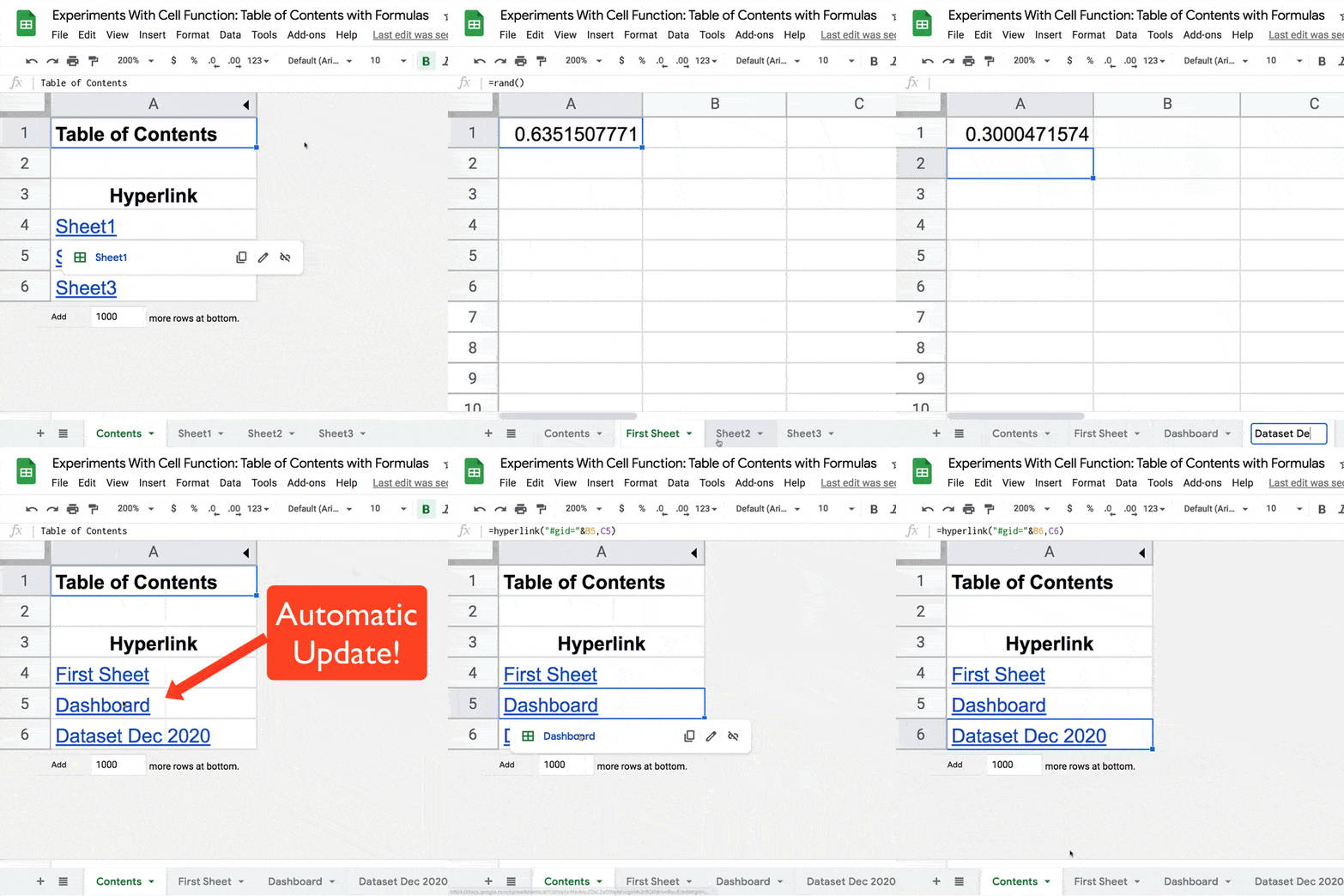
I’m going to use formulas to create a dynamic table of contents that updates automatically when you change the sheet names.

Formula Table Of Contents

The key to it all is the CELL function, which can extract the address of a cell.

Continue reading Experiments With Cell Function: Create A Dynamic Table Of Contents In Google Sheets With Formulas

Reverse Text In Google Sheets

In this example, you’ll see how to reverse text in Google Sheets.

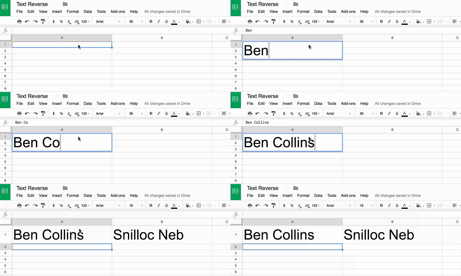
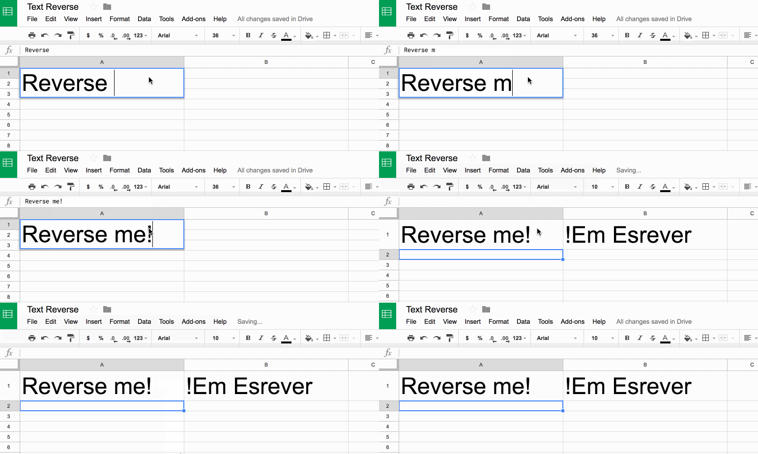
To start, enter some text into cell A1 and the formula in cell B1, to reverse the order of the text:

Text reverse in Google Sheets

Reverse Text In Google Sheets

What’s the formula?

=ArrayFormula(IFERROR(PROPER(CONCATENATE(MID(A1,LEN(A1)-ROW(INDIRECT("1:"&LEN(A1)))+1,1))),""))

It’s a beast! See below for a detailed breakdown of how it works.

It might be useful if you wanted to find the last character in a string, or the last occurrence of a character using the FIND() function.

Here’s an alternative, which reverses the capitalization too (submitted by Michael D over email – thanks!):

=JOIN("",ARRAYFORMULA(MID(A1,LEN(A1)-ROW(INDIRECT("1:"&LEN(A1)))+1,1)))

Can I see an example worksheet?

Yes, here you go.

How does this formula work?

Basically we make an array of numbers corresponding to how many letters are in the original text string. Then we reverse that, so the array shows the largest number first. Then we extract each letter at that position (so the largest number will extract the last letter, the second largest will extract the second-to-last letter, etc., all the way to the smallest number extracting the first letter). Then we concatenate these individual letters.

Easy! Err…

The only way to really understand this formula is to break it down, starting from the inner functions and building back out.

Assuming we have the text string “Abc” in cell A1, then let’s build the formula up in cell B1, step-by-step:

Step 1:

Use the LEN function to calculate the length of the text string and turn it into a range string with “1:”&LEN(A1)

Use the INDIRECT function to turn this string range reference into a valid range reference.

Finally wrap with ROW to convert into a row number list.

=ROW(INDIRECT("1:"&LEN(A1)))

which outputs a result of 1 in cell B1.

Step 2:

Turn the formula into an array formula, by hitting Ctrl + Shift + Enter, or Cmd + Shift + Enter (on a Mac), to the formula above. This will add the ArrayFormula wrapper around the formula:

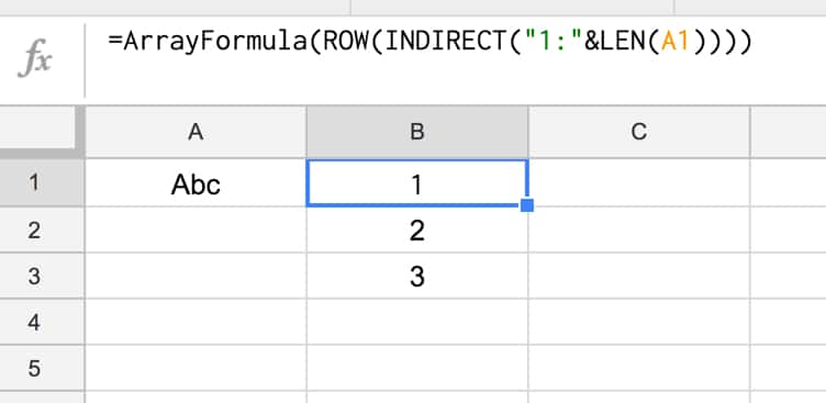
=ArrayFormula(ROW(INDIRECT("1:"&LEN(A1))))

This outputs 1 in cell B1, 2 in cell B2 and 3 in cell B3:

Array to reverse text

Step 3:

Reverse the output, so 3 is in cell B1, 2 in B2 and 1 in B3, by subtracting from the length of the text in A1 and adding 1 to avoid 0:

=ArrayFormula(LEN(A1)-ROW(INDIRECT("1:"&LEN(A1))) + 1)

Step 4:

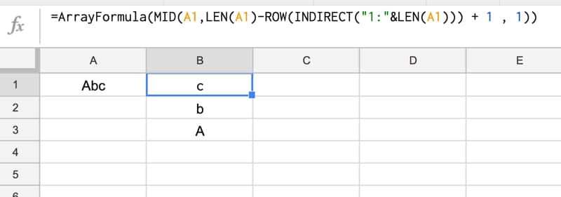
Use the MID formula to now extract the letters at position 3 (“c”), position 2 (“b”) and position 1 (“A”) and display in cells B1:B3:

=ArrayFormula(MID(A1,LEN(A1)-ROW(INDIRECT("1:"&LEN(A1))) + 1 , 1))

so your output is now:

MID formula in Google Sheets

Step 5:

Concatenate so that all the individual outputs are combined into a single cell:

=ArrayFormula(CONCATENATE(MID(A1,LEN(A1)-ROW(INDIRECT("1:"&LEN(A1))) + 1 , 1)))

Reverse text in google sheets

Step 6 (optional):

The string is essentially reversed now, so we could stop here.

However, you can use the PROPER function to capitalize the first letters of each word only, for a true reverse effect:

=ArrayFormula(PROPER(CONCATENATE(MID(A1,LEN(A1)-ROW(INDIRECT("1:"&LEN(A1))) + 1 , 1))))

Step 7 (optional):

Last step is to add in an IFERROR function to avoid an unsightly error message if the input cell (A1) is blank:

=ArrayFormula(IFERROR(PROPER(CONCATENATE(MID(A1,LEN(A1)-ROW(INDIRECT("1:"&LEN(A1)))+1,1))),""))

Final output:

Here’s the formula in action again:

Reverse text in google sheets

Further Reading

You might also like this article on Using Text Rotation to Create Custom Table Headers in Google Sheets.