Tag: Google Sheets

In this example, we’re going to see how to extract the first and last dates of the prior month, i.e. the last full month before this current one.

It’s the sort of date filter that’s frequently used in digital marketing, when you want to restrict your data to just web traffic or revenue in this period for comparison.

How do I get the first and last dates of the previous month?

We combine two functions, TODAY and EOMONTH, and a little bit of math to create the formulas to extract first and last dates.

What’s the formula?

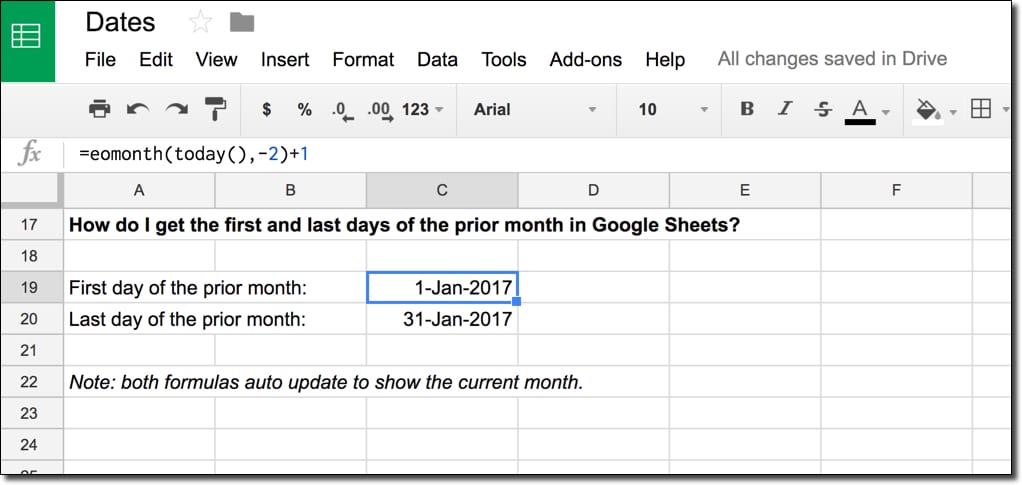
For the first day of the prior month:

For the last day of the prior month:

Can I see an example worksheet?

Yes, here you go.

How does this formula work?

The heart of both of these formulas is the function TODAY(), which outputs today’s date in your Sheet. It updates automatically whenever the spreadsheet is recalculated (when you make an edit somewhere else). It’s known as a volatile function because it automatically recalculates, so if you were to have a huge number of these formulas, it would affect the performance of your spreadsheet.

So we start with:

Next we wrap that with the EOMONTH function to get the date at the end of the month.

For the first day of the previous month, we offset by -2 to go back two months (which gives the last day of December in this example). To this we then add 1 day to nudge us into the first day of the previous month (January 2017 in this example), as follows:

The formula for the last day of the prior month is simpler. We offset -1 to go back one month and we don’t need to add a day to the output. So the formula is:

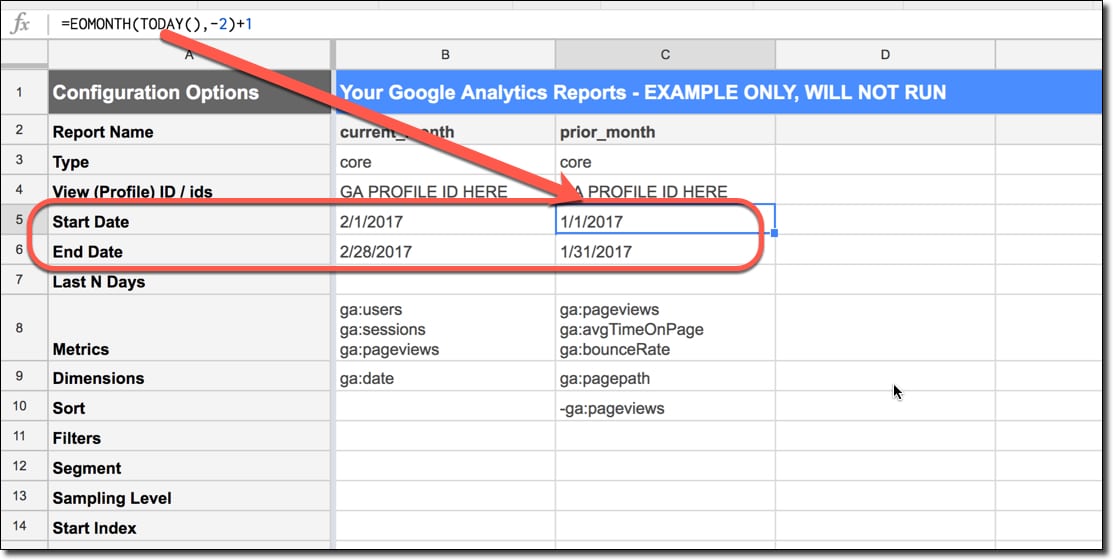
These types of date formulas are super useful if you do any data analysis work, and want to group and compare data for set periods. As an example, you may want to automatically generate Start and End Date fields in the Google Analytics Add-On, to always extract the most recent data for current and prior month periods for comparison.

See also: We can perform similar calculations to get weekly dates, prior months, quarterly dates and yearly dates.

Check out this article on creating a custom Google Analytics report in a Google spreadsheet, to see date formulas in action.

Have you ever wished the VLOOKUP function could return multiple columns?

For example, maybe you want to return several values that match a search term so that you can use a range of data as an input for another formula (e.g. a sparkline).

Of course, you could set up multiple vlookup formulas, but this wouldn’t work if you want to pass the data range into another formula, like the sparkline for example.

However, you can easily achieve it with just one formula.

Continue reading Have Vlookup Return Multiple Columns in Google Sheets

The VLOOKUP function is a super popular formula but suffers from a major drawback. You can’t lookup data to the left!

However, there’s a sneaky trick that lets us VLOOKUP to the left, so we can search for a term and return a result from a column to the left of the original search column:

Continue reading How To VLOOKUP To The Left In Google Sheets?