💡 Learn moreLearn how to write Apps Script and turbocharge your Google Workspace experience with the new Beginner Apps Script course
Google Sheets Macros are small programs you create inside of Google Sheets without needing to write any code.
They’re used to automate repeatable tasks. They work by recording your actions as you do something and saving these actions as a “recipe” that you can re-use again with a single click.
For example, you might apply the same formatting to your charts and tables. It’s tedious to do this manually each time. Instead you record a macro to apply the formatting at the click of a button.
In this article, you’ll learn how to use them, discover their limitations and also see how they’re a great segue into the wonderful world of Apps Script coding!
Think of a typical day at work with Google Sheets open. There are probably some tasks you perform repeatedly, such as formatting reports to look a certain way, or adding the same chart to new sales data, or creating that special formula unique to your business.
They all take time, right?
They’re repetitive. Boring too probably. You’re just going through the same motions as yesterday, or last week, or last month. And anything that’s repetitive is a great contender for automating.
This is where Google Sheets macros come in, and this is how they work:
Click a button to start recording a macro
Do your stuff
Click the button to stop recording the macro
Redo the process whenever you want at the click of a button
There’s the obvious reason that macros in Google Sheets can save you heaps of time, allowing you to focus on higher value activity.
But there’s a host of other less obvious reasons like: avoiding mistakes, ensuring consistency in your work, decreased boredom at work (corollary: increased motivation!) and lastly, they’re a great doorway into the wonderful world of Apps Script coding, where you can really turbocharge your spreadsheets and Google Workspace work.
Let’s run through the process of creating a super basic macro, in steps:
1) Open a new Google Sheet (pro-tip 1: type sheets.new into your browser to create a new Sheet instantly, or pro-tip 2: in your Drive folder hit Shift + s to create a new Sheet in that folder instantly).
Type some words in cell A1.
2) Go to the macro menu: Tools > Macros > Record macro
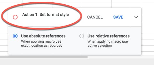
3) You have a choice between Absolute or Relative references. For this first example, let’s choose relative references:
Absolute references apply the formatting to the same range of cells each time (if you select A1:D10 for example, it’ll always apply the macro to these cells). It’s useful if you want to apply steps to a new batch of data each time, and it’s in the same range location each time.
Relative references apply the formatting based on where your cursor is (if you record your macro applied to cell A1, but then re-run the macro when you’ve selected cell D5, the macro steps will be applied to D5 now). It’s useful for things like formulas that you want to apply to different cells.
4) Apply some formatting to the text in cell A1 (e.g. make it bold, make it bigger, change the color, etc.). You’ll notice the macro recorder logging each step:
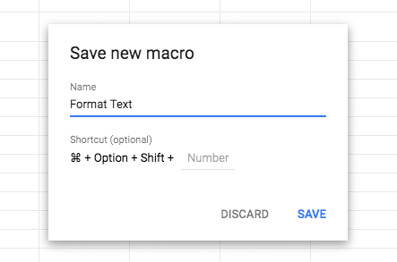
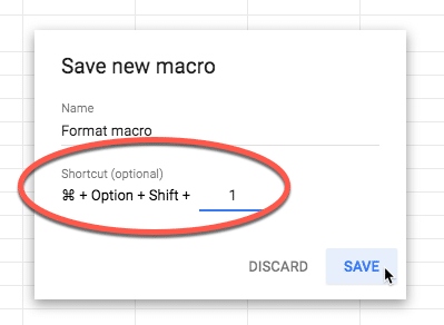
5) When you’ve finished, click SAVE and give your Macro a name:
(You can also add a shortcut key to allow quick access to run your macro in the future.)
Click SAVE again and Google Sheets will save your macro.
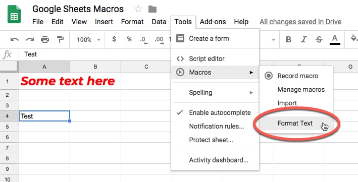
6) Your macro is now available to use and is accessed through the Tools > Macros menu:
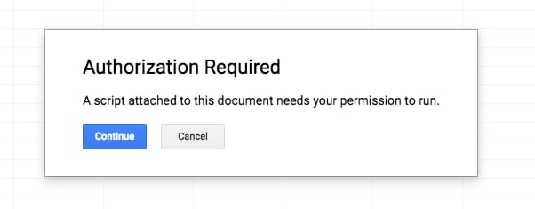
7) The first time you run the macro, you’ll be prompted to grant it permission to run. This is a security measure to ensure you’re happy to run the code in the background. Since you’ve created it, it’s safe to proceed.
First, you’ll click Continue on the Authorization popup:
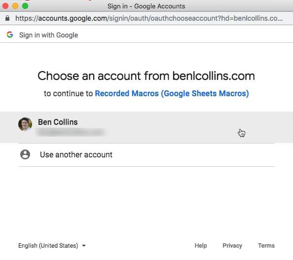
Then select your Google account:
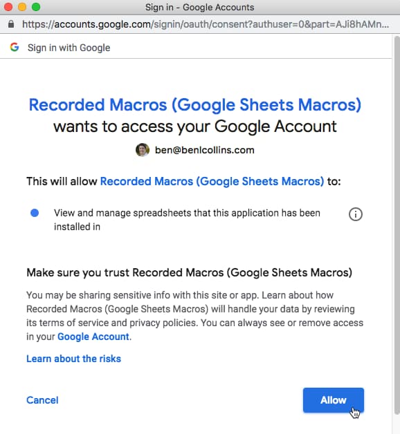
Finally, review the permissions, and click Allow:
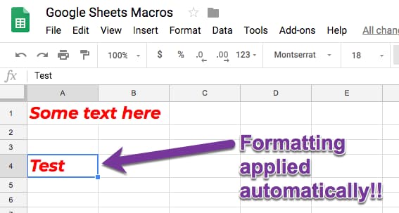
8) The macro then runs and repeats the actions you recorded on the new cell you’ve selected!
You’ll see the following yellow status messages flash across the top of your Google Sheet:
and then you’ll see the result:
Woohoo!
Congratulations on your first Google Sheets macro! You see, it was easy!
Here’s a quick GIF showing the macro recording process in full:
This is an optional feature when you save your macro in Google Sheets. They can also be added later via the Tools > Macros > Manage macros menu.
Shortcuts allow you to run your macros by pressing the specific combination of keys you’ve set, which saves you further time by not having to click through the menus.
Any macro shortcut keys must be unique and you’re limited to a maximum of 10 macro shortcut keys per Google Sheet.
In the above example, I could run this macro by pressing:
⌘ + option + shift + 1
keys at the same time (takes practice ?). Will be a different key combo on PC/Chromebooks.
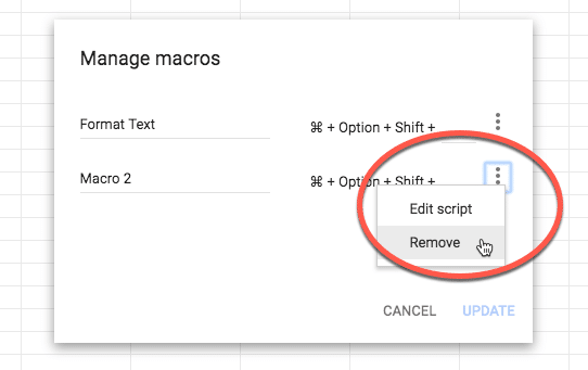
4.2 Deleting macros
You can remove Google Sheets macros from your Sheet through the manage macros menu: Tools > Macros > Manage macros
Under the list of your macros, find the one you want to delete. Click the three vertical dots on right side of macro and then choose Remove macro:
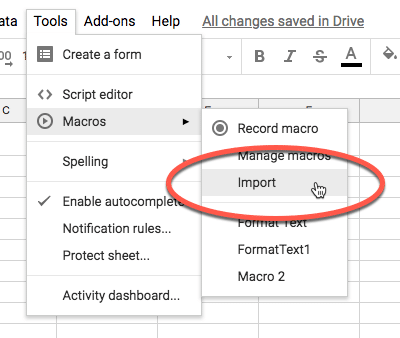
4.3 Importing other macros
Lastly, you can add any functions you’ve created in your Apps Script file to the Macro menu, so you can run them without having to go to the script editor window. This is a more advanced option for users who are more comfortable with writing Apps Script code.
This option is only available if you have functions in your Apps Script file that are not already in the macro menu. Otherwise it will be greyed out.
Use the minimum number of actions you can when you record your macros to keep them as performant as possible.
For macros that make changes to a single cell, you can apply those same changes to a range of cells by highlighting the range first and then running the macro. So it’s often not necessary to highlight entire ranges when you’re recording your macros.
Macros are bound to the Google Sheet in which they’re created and can’t be used outside of that Sheet. Similarly, macros written in standalone Apps Script files are simply ignored.
Macros are not available for other Google Workspace tools like Google Docs, Slides, etc. (At least, not yet.)
You can’t distribute macros as libraries or define them in Sheets Add-ons. I hope the distribution of macros is improved in the future, so you can create a catalog of macros that is available across any Sheets in your Drive folder.
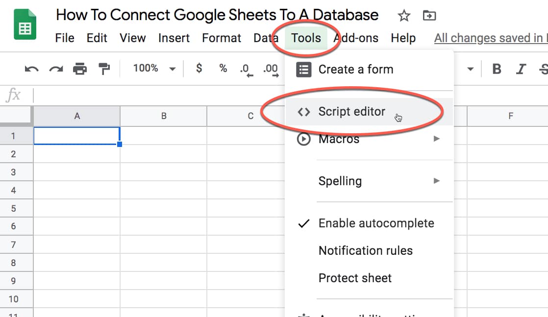
If you want to take a look at this code, you can see it by opening the script editor (Tools > Script editor or Tools > Macros > Manage macros).
You’ll see an Apps Script file with code similar to this:
/** @OnlyCurrentDoc */

function FormatText() {
  var spreadsheet = SpreadsheetApp.getActive();
  spreadsheet.getActiveRangeList().setFontWeight('bold')
  .setFontStyle('italic')
  .setFontColor('#ff0000')
  .setFontSize(18)
  .setFontFamily('Montserrat');
};
Essentially, this code grabs the spreadsheet and then grabs the active range of cells I’ve selected.
The macro then makes this selection bold (line 5), italic (line 6), red (line 7, specified as a hex color), font size 18 (line 8), and finally changes the font family to Montserrat (line 9).
The video at the top of this page goes into a lot more detail about this Apps Script, what it means and how to modify it.
Macros in Google Sheets are a great first step into the world of Apps Script, so I’d encourage you to open up the editor for your different macros and check out what they look like.
(In case you’re wondering, the line /** @OnlyCurrentDoc */ ensures that the authorization procedure only asks for access to the current file where your macro lives.)
Record the steps as you format your reporting tables, so that you can quickly apply those same formatting steps to other tables. You’ll want to use Relative references so that you can apply the formatting wherever your table range is (if you used absolute then it will always apply the formatting to the same range of cells).
Check out the video at the top of the page to see this example in detail, including how to modify the Apps Script code to adjust for different sized tables.
8.2 Creating charts
If you find yourself creating the same chart over and over, say for new datasets each week, then maybe it’s time to encapsulate that in a macro.
Record your steps as you create the chart your first time so you have it for future use.
The video at the top of the page shows an example in detail.
The following macros are intended to be copied into your Script Editor and then imported to the macro menu and run from there.
8.3 Convert all formulas to values on current Sheet
Open your script editor (Tools > Script editor). Copy and paste the following code onto a new line:
// convert all formulas to values in the active sheet
function formulasToValuesActiveSheet() {
  var sheet = SpreadsheetApp.getActiveSheet();
  var range = sheet.getDataRange();
  range.copyValuesToRange(sheet, 1, range.getLastColumn(), 1, range.getLastRow());
};
Back in your Google Sheet, use the Macro Import option to import this function as a macro.
When you run it, it will convert any formulas in the current sheet to values.
8.4 Convert all formulas to values in entire Google Sheet
Open your script editor (Tools > Script editor). Copy and paste the following code onto a new line:
// convert all formulas to values in every sheet of the Google Sheet
function formulasToValuesGlobal() {
  var sheets = SpreadsheetApp.getActiveSpreadsheet().getSheets();
  sheets.forEach(function(sheet) {
    var range = sheet.getDataRange();
    range.copyValuesToRange(sheet, 1, range.getLastColumn(), 1, range.getLastRow());
  });
};
Back in your Google Sheet, use the Macro Import option to import this function as a macro.
When you run it, it will convert all the formulas in every sheet of your Google Sheet into values.
8.5 Sort all your sheets in a Google Sheet alphabetically
Open your script editor (Tools > Script editor). Copy and paste the following code onto a new line:
// sort sheets alphabetically
function sortSheets() {
  var spreadsheet = SpreadsheetApp.getActiveSpreadsheet();
  var sheets = spreadsheet.getSheets();
  var sheetNames = [];
  sheets.forEach(function(sheet,i) {
    sheetNames.push(sheet.getName());
  });
  sheetNames.sort().forEach(function(sheet,i) {
    spreadsheet.getSheetByName(sheet).activate();
    spreadsheet.moveActiveSheet(i + 1);
  });
};
Back in your Google Sheet, use the Macro Import option to import this function as a macro.
When you run it, it will sort all your sheets in a Google Sheet alphabetically.
8.6 Unhide all rows and columns in the current Sheet
Open your script editor (Tools > Script editor). Copy and paste the following code onto a new line:
// unhide all rows and columns in current Sheet data range
function unhideRowsColumnsActiveSheet() {
  var sheet = SpreadsheetApp.getActiveSheet();
  var range = sheet.getDataRange();
  sheet.unhideRow(range);
  sheet.unhideColumn(range);
}
Back in your Google Sheet, use the Macro Import option to import this function as a macro.
When you run it, it will unhide any hidden rows and columns within the data range. (If you have hidden rows/columns outside of the data range, they will not be affected.)
8.7 Unhide all rows and columns in entire Google Sheet
Open your script editor (Tools > Script editor). Copy and paste the following code onto a new line:
// unhide all rows and columns in data ranges of entire Google Sheet
function unhideRowsColumnsGlobal() {
  var sheets = SpreadsheetApp.getActiveSpreadsheet().getSheets();
  sheets.forEach(function(sheet) {
    var range = sheet.getDataRange();
    sheet.unhideRow(range);
    sheet.unhideColumn(range);
  });
};
Back in your Google Sheet, use the Macro Import option to import this function as a macro.
When you run it, it will unhide any hidden rows and columns within the data range in each sheet of your entire Google Sheet.
8.8 Set all Sheets to have a specific tab color
Open your script editor (Tools > Script editor). Copy and paste the following code onto a new line:
// set all Sheets tabs to red
function setTabColor() {
  var sheets = SpreadsheetApp.getActiveSpreadsheet().getSheets();
  sheets.forEach(function(sheet) {
    sheet.setTabColor("ff0000");
  });
};
Back in your Google Sheet, use the Macro Import option to import this function as a macro.
When you run it, it will set all of the tab colors to red.
Want a different color? Just change the hex code on line 5 to whatever you want, e.g. cornflower blue would be 6495ed
Open your script editor (Tools > Script editor). Copy and paste the following code onto a new line:
// remove all Sheets tabs color
function resetTabColor() {
  var sheets = SpreadsheetApp.getActiveSpreadsheet().getSheets();
  sheets.forEach(function(sheet) {
    sheet.setTabColor(null);
  });
};
Back in your Google Sheet, use the Macro Import option to import this function as a macro.
When you run it, it will remove all of the tab colors from your Sheet (it sets them back to null, i.e. no value).
Here’s a GIF showing the tab colors being added and removed via Macros (check the bottom of the image):
8.10 Hide all sheets apart from the active one
Copy and paste this code into your script editor and import the function into your Macro menu:
function hideAllSheetsExceptActive() {
  var sheets = SpreadsheetApp.getActiveSpreadsheet().getSheets();
  sheets.forEach(function(sheet) {
    if (sheet.getName() != SpreadsheetApp.getActiveSheet().getName())
      sheet.hideSheet();
  });
};
Running this macro will hide all the Sheets in your Google Sheet, except for the one you have selected (the active sheet).
8.11 Unhide all Sheets in your Sheet in one go
Open your script editor (Tools > Script editor). Copy and paste the following code onto a new line:
function unhideAllSheets() {
  var sheets = SpreadsheetApp.getActiveSpreadsheet().getSheets();
  sheets.forEach(function(sheet) {
    sheet.showSheet();
  });
};
Back in your Google Sheet, use the Macro Import option to import this function as a macro.
When you run it, it will show any hidden Sheets in your Sheet, to save you having to do it 1-by-1.
Here’s a GIF showing how the hide and unhide macros work:
You can see how Sheet6, the active Sheet, is the only one that isn’t hidden when the first macro is run.
8.12 Resetting Filters
Ok, saving the best to last, this is one of my favorite macros! 🙂
I use filters on my data tables all the time, and find it mildly annoying that there’s no way to clear all your filters in one go. You have to manually reset each filter in turn (time consuming, and sometimes hard to see which columns have filters when you have really big datasets) OR you can completely remove the filter and re-add from the menu.
Let’s create a macro in Google Sheets to do that! Then we can be super efficient by running it with a single menu click or even better, from a shortcut.
Open your script editor (Tools > Script editor). Copy and paste the following code onto a new line:
// reset all filters for a data range on current Sheet
function resetFilter() {
  var sheet = SpreadsheetApp.getActiveSheet();
  var range = sheet.getDataRange();
  range.getFilter().remove();
  range.createFilter();
}
Back in your Google Sheet, use the Macro Import option to import this function as a macro.
When you run it, it will remove and then re-add filters to your data range in one go.
Here’s a GIF showing the problem and macro solution:
Access Apps Script under the menu Tools > Script editor
2) Replace “Code.gs” with the code here. (Skip this if you copied the Sheet above)
3) We included credentials for SeekWell’s demo MySQL database. To connect to your database, replace the six fields below. Note you’ll need to whitelist Google’s IP addresses.
var HOST = 'yourhostname'

var PORT = '3306 or your port'

var USERNAME = 'yourusername'

var PASSWORD = 'yourpassword'

var DATABASE = 'youdatabasename'

var DB_TYPE = 'mysql or your type'
4) You might also want to change the MAXROWS, but you don’t go too crazy, Sheets has a hard limit of 10 million cells and the query will take longer to run with more rows.
5) Save the file and refresh / refresh the Sheet. You’ll see a new menu option of “SeekWell Lite” show up.
6) The script is set up to read the query from query!A2 and write the results to your active cell, so you’ll need to add a sheet called “query” and add the query below in the cell query!A2 (skip if you copied the Sheet above).
SELECT *

FROM dummy.users

LIMIT 100
7) Go back to Sheet1, click in cell C4 (or any other cell) and click “SeekWell Lite” → “Run SQL”.
In a few moments you’ll see the data show up!
A few problems with this approach
You need to store your password in plain text in the Code.gs file.
Sharing the script with your team and adding the script to different Sheets is a bit of a pain. You can publish an addon, but that comes with some overhead.
And scheduling / automating refreshes can be cumbersome when you need many different queries going to many different Sheets.
Google’s JDBC service doesn’t work for Postgres, Snowflake or RedShift and requires a long list of whitelisted IP’s. It also doesn’t support SSH.
Alternatives to Google Sheets database connections with App Script
A lot of people hate paying for things they can do for free, but you should always do some napkin math when making the “build vs. buy” decision.
In the case of automating reports, the ROI can be pretty high, especially if you have several daily, hourly, or near real time dashboards you need to keep updated. ActionDesk did a good overview of the options out there.
This is a guest post written by Mike Ritchie. Mike is the co-founder of Seekwell and has over 15 years experience in analytics.
SeekWell features include:
Takes < 2 minutes to get your first schedule set up
A shared code repository with every query anyone on your team has ever written
Beautiful query editor with autocomplete and snippets
Mastering Google Sheets formulas is more than just knowing the functions themselves and how to combine them.
True mastery comes when you know all of the little, hidden shortcuts and tricks built in to Google Sheets to help you with your formulas. Individually they may not seem like much, but combine them together in your toolkit and you’ll be more efficient and effective when working with Google spreadsheet formulas.
How many of these Google Sheets Formulas Tips & Techniques do you know?
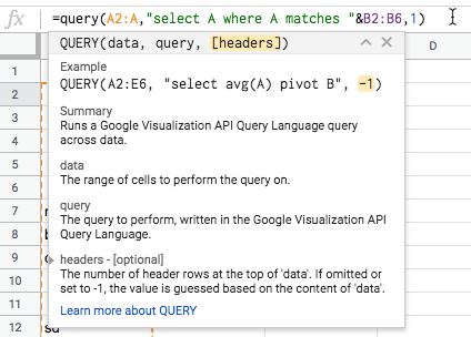
You can press the “X” to remove the whole pane if it’s getting it the way. Or you can minimize/maximize with the arrow in the top right corner.
The best feature of the formula pane is the yellow highlighting it adds to show you which section of your function you are in. E.g. in the image above I’m looking at the “[headers]” argument.
There is information about what data the function is expecting and even a link to the full Google documentation for that function.
If you’ve hidden the function pane, or you can’t see it, look for the blue question mark next to the equals sign of your formula. Click that and it will restore the function helper pane.
Helpfully Google Sheets highlights ranges in your formulas and in your actual Sheet with matching colors. It applies different colors to each unique range in your formula.
8. F2 To Highlight Specific Ranges In Your Google Sheets Formulas
As mentioned in Step 2, you press the F2 key to enter the formula view of a cell with a formula in.
However, it has another useful property. If you position your cursor over a range of data in your formula and then press the F2 key, it will highlight that range of data for you:
When you’re using the function drop-down list in the tip above, press the tab key to auto-complete the function name (based on whatever function is highlighted).
An easy one this! Grab the base of the formula bar until you see the cursor change into a little double-ended arrow. Then click and drag down to make the formula bar as wide as you want.
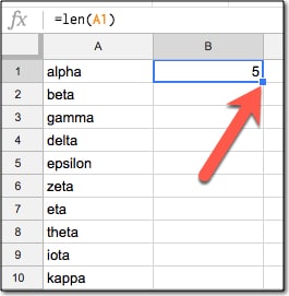
To copy the formula quickly down the column, double-click the blue mark in the corner of the highlighted cell, shown by the red arrow. This will copy the cell contents and format down as far as the contiguous range in preceding column (column A in this case).
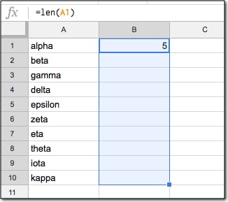
An alternative way to quickly fill in a column is to highlight the range you want to fill, e.g.:
Then press Ctrl + D (PC and Chromebook) or Cmd + D (Mac) to copy the contents and format down the whole range, like so:
You can also do this with Ctrl + Enter (PC and Chromebook) or Cmd + Enter (Mac), which will fill down the column.
Array Formulas in Google Sheets are powerful extensions to regular formulas, allowing you to work with ranges of data rather than individual pieces of data.
Per the official definition, array formulas enable the display of values returned into multiple rows and/or columns and the use of non-array functions with arrays.
In a nutshell: whereas a normal formula outputs a single value, array formulas output a range of cells!
We need to tell Google Sheets we want a formula to be an Array Formula. We do this in two ways:
Hit Ctrl + Shift + Enter (PC/Chromebook) or Cmd + Shift + Enter (on a Mac) and Google Sheets will add the ArrayFormula wrapper
Alternatively, type in the word ArrayFormula and add brackets to wrap your formula
Have you ever used the curly brackets, or ARRAY LITERALS to use the correct nomenclature, in your formulas?
An array is a table of data. They can be used in the same way that a range of rows and columns can be used in your formulas. You construct them with curly brackets:
{ }
Commas separate the data into columns on the same row.
Semi-colons create a new row in your array.
(Please note, if you’re based in Europe, the syntax is a little different. Find out more here.)
This formula, entered into cell A1, will create a 2 by 2 array that puts data in the range A1 to B2:
= { 1 , 2 ; 3 , 4 }
The array component (in this example { 1 , 2 ; 3 , 4 } ) can be used as an input to other formulas.
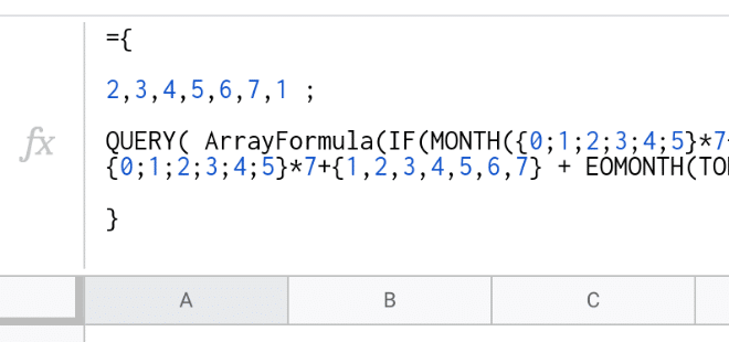
Press Ctrl + Enter inside the formula editor bar to add new lines to your formulas, to make them more readable. Note, you’ll probably want to widen the formula bar first, per tip 11.
If you’re building complex formulas, then I advocate a one-action-per-step approach. What I mean by this is build your formula in a series of steps, and only make one change with each step. So if you start with function A(range) in a cell, then copy it to a new cell before you nest it with B(A(range)), etc.
This lets you progress in a step-by-step manner and see exactly where your formula breaks down.
Similarly, if you’re trying to understand complex formulas, peel the layers back until you reach the core (which is hopefully a position you understand). Then, build it back up in steps to get back to the full formula.
For more detail about this approach, including examples and worksheets for each case, have a read of this post:
This Google Sheets tutorial will help take you from an absolute beginner, or basic user, through to a confident, competent, intermediate-level user.
Google Sheets is a hugely powerful tool, for everything from digital marketing to finance modeling, from project management to statistical analysis, in fact, just about any activity involving the recording and analysis of data.
And if you’re (relatively) new, it really pays dividends to learn how to use Google Sheets correctly. This tutorial will help you transition from newbie to ninja in short order!
If you’re new to Google Sheets, then I recommend you start from the beginning of this article.
However, if you’ve used Sheets before, feel free to skip sections 1 and 2, and begin with the Data and basic formulas section.
A template is available for copying to your Drive, to accompany this tutorial:
💡 Learn more Google Sheets Essentials is my new beginner’s course. It’s 100% online, on-demand video training course designed to boost your spreadsheet skills.
1. How to use Google Sheets
What is Google Sheets?
Google Sheets is a free, cloud-based spreadsheet application. That means you open it in your browser window like a regular webpage, but you have all the functionality of a full spreadsheet application for doing powerful data analysis. It really is the best of both worlds.
How is it different to Excel?
No doubt you’ve heard of Microsoft Excel, the long-established heavyweight of the spreadsheet world. It’s an incredibly powerful, versatile piece of software, used by approximately 750 million – 1 billion people worldwide. So yeah, a tough act to follow.
Google Sheets is similar in many ways, but also distinctly different in other areas. It has (mostly) the same set of functions and tools for working with data. In fact, some people mistakenly call it “Google Excel” or “Google spreadsheets.”
With the risk of getting into an opinionated debate about the strengths/weaknesses of each platform, here are a few key differences:
Google Sheets is cloud-based whereas Excel is a desktop program. With Sheets, you’ll no longer have versions of your work floating around. Everyone always sees the same, most up-to-date version of Sheets, showing the same spreadsheet data.
Collaboration is baked into Sheets, so it works extremely well. Excel is still trying to play catch up here.
Both have charting tools and Pivot Table tools for data analysis, although Excel’s are more powerful in both cases.
Excel can handle much bigger datasets than Sheets, which has a limit of 10 million cells.
Being a cloud-based program, Google Sheets integrates really well with other online Google services and third-party sites.
Both have scripting languages to extend their functionality and build custom tools. Google Sheets uses Apps Script (a variant of Javascript) and Excel uses VBA.
For the material we’ll cover in this article, there’s very little difference between the programs, however.
For a deep-dive into the differences between Excel and Google Sheets, have a look at ExcelToSheets.com
Why use Google Sheets?
How’s this for starters:
It’s free!
It’s collaborative, so teams can all see and work with the same spreadsheet in real-time.
It has enough features to do complex analysis, but…
…it’s also really easy to use.
Need more convincing? Here are 5 more reasons from Google themselves.
Can it still do advanced stuff?
Absolutely! You can build dashboards, write formulas that make your head spin and even build applications to automate your job. The sky’s the limit!
You’ll find lots of resources on this site for intermediate/advanced level users, as well as comprehensive online training courses.
Ok, where do I get it? How to create your first Google Sheet
Click on the Go To Google Sheets button in the middle of the screen. You’ll be prompted to login:
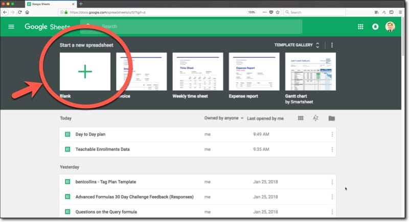
And then you arrive at the Google Sheets home screen, which will show any previous spreadsheets you’ve created.
Click the huge green plus button to create a new Google Sheet:
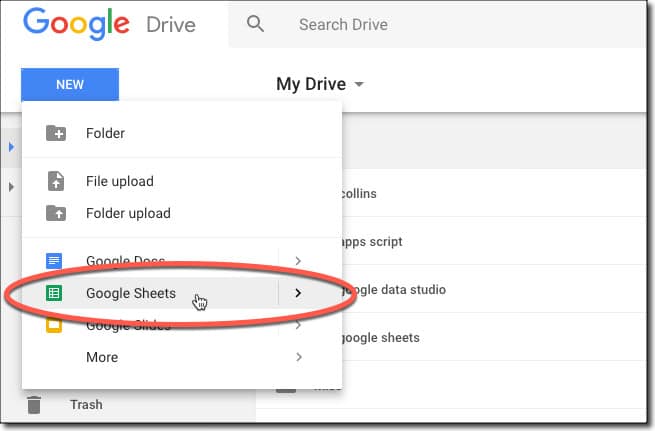
Opening your first Google Sheet from Drive
You can create new Google Sheets from your Drive folder by clicking on the blue NEW button:
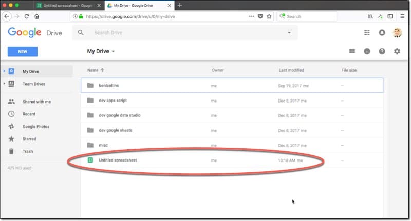
When you create a new Google Sheet, it’ll be created in your main Drive folder (your root folder):
(Note: Don’t panic if you don’t see the Sheet yet, it may not show up until you’ve renamed it. See next step on how to do this.)
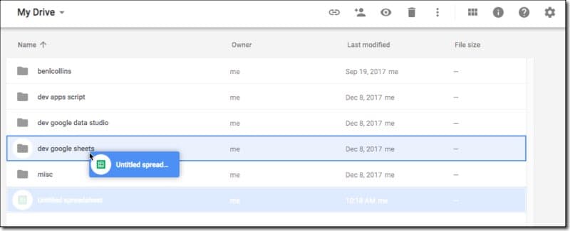
Here you can drag it to a different folder if you wish (to keep things organized). Do this by clicking-and-holding the file, and dragging to where you want it to go:
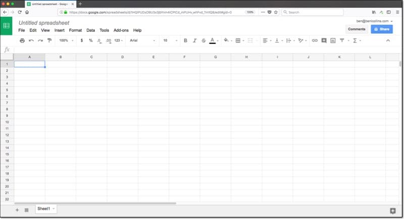
The Google Sheet editing window
This is what your blank Google Sheet will look like:
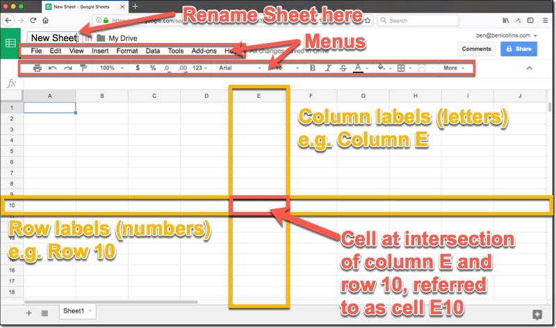
You can rename your Sheet in the top left corner. Click on where it says Untitled spreadsheet and type in whatever name you want to give your Sheet, in this example “New Sheet”.
So let’s introduce some key terminology and the fundamental concept upon which spreadsheets work:
There are two menu rows above your Sheet, of which we’ll see more further on in this tutorial.
The main window consists of a grid of cells. An individual cell is a single rectangle, at the intersection of one column and one row, and it’ll hold a single piece of data.
The columns are vertical ranges of cells, labeled by letters running across the top of the Sheet.
Rows are horizontal ranges of cells, labeled by numbers running down the left side of your Sheet.
In the example above, I highlighted column E and row 10.
** The fundamental concept of spreadsheets: **
Column E and row 10 intersect at one cell, and one cell only. Thus we can combine the column letter and row number to create a unique reference to this cell, E10. Now when we want to refer to this cell, for example to access data in this cell, we use the address E10 to do that.
Understand this and you understand spreadsheets. The rest is just details!
Entering, selecting, deleting and moving data
Now the fun really starts! Let’s start using this new blank sheet we’ve created.
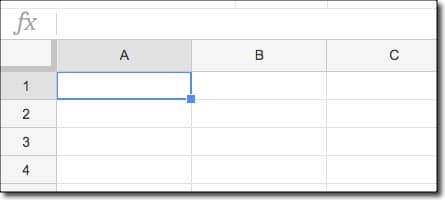
Click cell A1 (that’s the intersection of column A with row 1, the cell in the top left corner of the Sheet) and you’ll see a blue box around the cell, to indicate it’s highlighted:
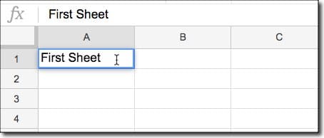
Then you can simply start typing and you’ll see the data being entered into that cell:
Hit enter when you’ve finished entering data and you’ll move down to the next cell, having completed your data entry. If you hit the Tab key instead, you’ll move across one cell to the right!
It’s worth pointing out an important nuance here:
Clicking ONCE on the cell highlights the whole cell. Clicking TWICE enters into the cell, so you can select or work with the data only.
If you find yourself stuck inside a cell, you can press the ESCAPE key to deselect the contents and go up a level, to just having the cell selected.
Try it for yourself and see how the cursor shows up inside the cell when you double-click, allowing you to edit the data.
To delete the data we just entered, either click the cell once and hit the delete key, or, click the cell twice and then press the delete key until all your data is cleared out.
💡 Learn more Check out my brand new beginner’s course: Google Sheets Essentials. This is a 100% online, on-demand video training course designed specifically to help you boost your spreadsheet skills.
Help! I made a mistake
First of all, don’t panic!
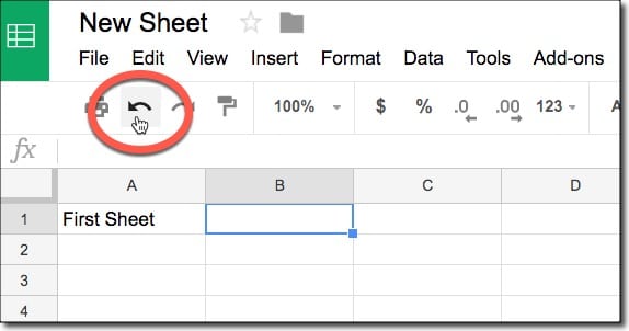
Google Sheets saves every step of your work so you can always go back a step (or two) if needed.
Press Cmd + Z if you’re on a Mac, or Ctrl + Z if you’re on a PC and you’ll undo your previous step. Keep pressing and you’ll simply go further back through your changes. (Pressing Cmd + Y on a Mac, or Ctrl + Y on a PC moves your forwards, to redo your last step.)
You can also undo using the Undo arrow on the menu:
Creating a basic table
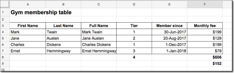
Right, with all that in mind, it’s time for a quick exercise.
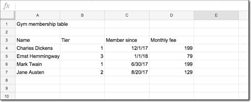
See if you can create the following table for our fictitious gym membership site, by entering the data into the correct cells (there is no formatting or other tricks used at this stage):
Feel free to use your own data if you wish. Also note that the dates entered above are in US format, with the Month first, so don’t worry if your table has the Day first.
2. How to use Google Sheets: The working environment
Changing the size, inserting, deleting, hiding/unhiding of columns and rows
To select a row or column, click on the number (rows) or letter (columns) of the row or column you want to select. This will highlight the whole row or column blue, to indicate you have it selected.
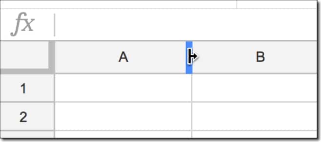
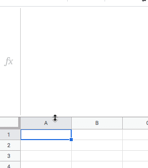
To change the width of a column, or height of a row, hover your cursor over the grey line denoting the edge of the column or row, until your cursor changes to look like this:
Then click and drag the cursor left or right to change the width of this column. It’s the same process to change the height of rows.
Pro-tip: To quickly change the column width to fit your cell contents, double-click when you’ve hovered over the grey line.
How to add columns in Google Sheets: To insert additional columns or rows, click on the existing column or row next to where you’d like to insert a new column or row. With the column or row selected (highlighted blue), right-click to bring up the options menu, then select Insert Before (or Insert After) for Columns, or Insert Above (or Insert Below) for Rows:
Adding extra rows and columns at end
If you reach the outer edges of a Google Sheet, you’ll notice the rows and/or columns stop. But don’t worry, you can add more.
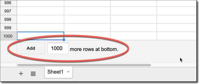
If you’ve scrolled all the way to the bottom of your Sheet (or added that much data), you’ll notice that you’re given 1,000 rows by default. There’s a button to add more rows if you need, either 1,000 as shown, or any number you wish (up to a limit, more on that below).
If you reach the right edge of the Sheet, i.e. the last column, then you add more columns in the standard way. Right-click a cell in the last column to bring up the menu and then choose to add a column to the right.
Pro-tip: If you want to add more than one column, there’s a trick to do it in one go. As an example, say you wanted to add three new columns to the right side of your Sheet, begin by highlighting the last three columns that are there already, then right-clicking and choosing to insert new columns. It’ll then insert three new columns for you!
Data Limit: Finally, keep in mind that each Google Sheet is limited to 10 million cells, which sounds like a lot but soon fills up. Anyway, you’ll find Sheets slows down considerably before reaching that limit. Most people report a slight slow down with tens of thousands of rows of data and complex formulas and models.
Adding/removing multiple sheets, renaming them
Super easy!
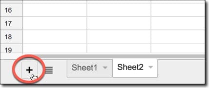
Click the big plus button in the bottom left of your Google Sheet to add a new Sheet (also called a Tab).
Why use multiple tabs within your Google Sheet?
Well, like a book with chapters on different topics, it can help separate different data and keep your Sheet organized.
For example, you might have a Sheet solely to record your global settings (any variables like name, email, tax rate, headcount…) and another for transactional data, and yet another for the analysis and charts.
The button with the three bars, next to the plus, is your index button, listing all of the tabs in your Google Sheet. This is super useful when you start having a lot of different tabs to manage.
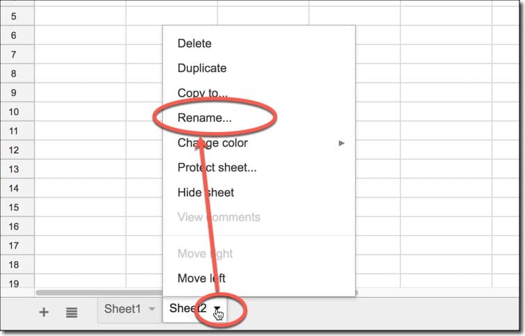
To rename a sheet, or delete a sheet, click the small arrow next to the name (e.g. Sheet1) to bring up the menu. Here you’ll see the option to rename, to delete, or even hide (and unhide) Sheets.
For naming, I try to indicate what’s in that tab, so use names like Settings, Dashboard, Charts, Raw Data.
Formatting
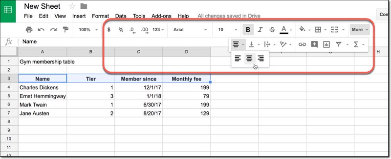
You’ll find all of the formatting options on the top toolbar, so you can center your headings, make them bold, format numbers as currency etc. You may find them all on one single row, or you may find some under the More button, as shown in this image:
They’re similar to a word processor and pretty self-explanatory. You can always hit undo if you make a mistake (Cmd + Z on Mac, or Ctrl + Z on PC).
Try the following to format our basic table:
> Make the heading bold and size 14px
> Center the column headings and make them bold
> Center the tier column
> Change the date format to 01-Jan-2018 (Hint: the date format is found under the button that says 123.)
> Add a dollar sign, $, to the fee column
> Add a border around the whole table.
Here’s a GIF to guide you:
(Note, you can also find the formatting options under the Format menu, between the Insert and Data menu options.)
Alternating colors
Let me show you the option to add alternating row colors (banding) to your tables.
Let’s apply it to our basic table, by highlighting the table and then from the menu:
Format > Alternating colors
as shown here:
Remember, a little bit of formatting goes a long way. If you Sheet is more readable and tidy, people will be more likely to understand it and absorb the information.
Removing formatting
This is my number 1 productivity tip in Google Sheets.
To remove all formatting from a cell (or range of cells), hit Cmd + \ on a Mac or Ctrl + \ on a PC.
This will save you so much time when you’re wanting to remove formatting that isn’t yours or that you no longer want or need.
3. How to use Google Sheets: Data and basic formulas
Different types of data
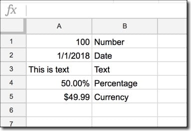
You’ve already seen different data types in Google Sheets in our basic table.
The key point to understand with spreadsheet data is that each cell contains the data itself, and a format applied to that data.
For example, suppose a cell contained:
2, or 2.00, or $2, or $2.00
In each case the underlying data is the number 2, but with a different format applied each time. If we add 2 to each of these cells we get back the number 4 in every case (with formatting applied).
Basic data types in Google Sheets
You’ll notice that currency data, percentage data and even dates are actually just numbers under the hood (dates? Really? Yes, they are, but that’s a discussion for another day). They’re all right-aligned, hanging out on the right edge of their cell.
Text is left-aligned by default.
If you want to force something to be stored as text, you can prepend a single quote, ' before the cell contents. So typing in '0123 will show as 0123 in your cell and be left-aligned. If you omit the single quote mark, then it’ll be stored as a number and show up as 123 without the 0.
Doing math on numbers
Easy-peasy, just like you do on a calculator.
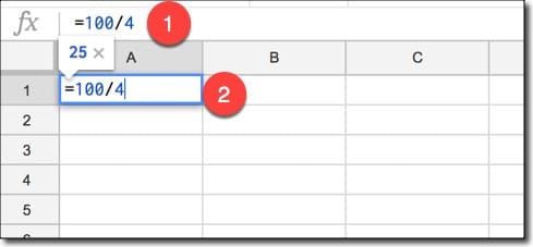
You click the cell you want to do your calculation in, type an equals sign (=) to indicate you’re performing a calculation and then type in your formula, e.g.
Notice how calculation will show in the formula bar (1) as well as in the cell (2).
You’ll notice that you get a preview of the answer (in this case, 25) above the formula.
Starting with functions: COUNT, SUM, AVERAGE
Technically you’ve already written your first formula in the section above on math calculations, but really, your formula career begins when you start using the built-in functions (of which there are hundreds!).
Returning to our basic table, let’s count how many members we have, what the total monthly fees are and what the average monthly fees are.
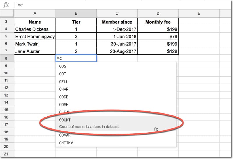
COUNT
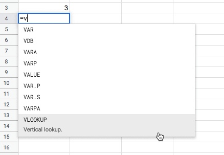
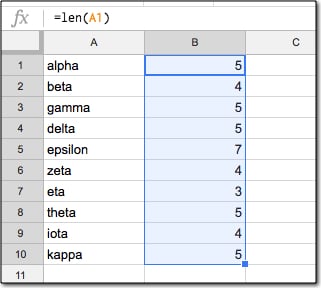
Click on cell B8, type an equals (=) and then start typing the word COUNT. You’ll notice an auto-complete menu comes up showing all of the functions beginning with C, like this:
You can either keep typing COUNT in full, or find it and select in from the list (hover over it and click on it OR hit enter OR hit tab).
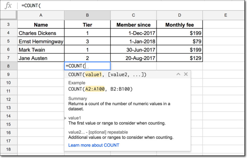
Next you’ll see the formula helper window show up, which tells you about the formula syntax and how to fill it in correctly:
In this case, the COUNT function is expecting a list of numeric values.
You have to select the range of cells you want to count. So click on B4, hold you mouse down and drag down to B7, so that the four cells are highlighted in orange and B4:B7 is showing up in your function:
Then, close the function with a closing bracket “)”:
=COUNT(B4:B7)
Note: COUNT is used to count numbers. If you want to count text (for example the names) then COUNT won’t work (it’ll give you a 0). Instead use COUNTA (with an A at the end), otherwise the method is the same.
SUM
Your turn! Try creating a total for the membership fees in cell D8. Follow the same process as the count function, except use SUM and highlight the values in column D.
=SUM(D4:D7)
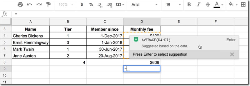
AVERAGE
You’re on a roll, so go ahead and calculate the average of the membership fees. Use the AVERAGE function in cell D9.
=AVERAGE(D4:D7)
Psst, you’ll notice that Google even helps you out sometimes and suggests the exact formula you were after:
Here you go:
If you make a mistake with your formula, you’ll see an errors message, probably something like #N/A, #REF!, #DIV/0 etc.
You’ll need to re-enter your formula and correct it before proceeding. These error messages do give a lot of context though, so they’re worth understanding.
What’s the difference between a function and a formula?
Well, both are used interchangeably and rather loosely so I wouldn’t get hung up on it.
For the pedantic, a function refers to the single method word (e.g. SUM) whereas a formula refers to the whole operation after the equals sign, often consisting of multiple functions.
Separating data with the Text to columns feature
Let’s suppose you wanted First Name and Last Name, rather than just simply Name as we have in our dead famous authors membership table. How do we go about doing that?
Well of course, as with everything in spreadsheets, there are lots of ways, but let me show you the easiest, using the Text to Columns feature.
Back to our basic table, create a new column to the right of Name before the Tier column, i.e. create a new, blank column B.
Highlight the four names and click:
Data > Split text to columns…
On the sub-menu that shows up choose SPACE and marvel at how Google Sheets separates the full name into a first and last name. Feel free to rename the columns First Name and Last Name too.
Combining cells
Oh, blast I hear you say! You meant to keep hold of that full Name column as well.
No problem, let’s learn how to combine text so we can rebuild it.
Insert a new blank column between B and C (between Last name and Tier) and call it Full Name, in cell C3.
Add this formula in cell C4:
= A4 & B4
That’s A4, Ampersand, B4.
What it does is combine the data in cell A4 with the data in cell B4 and output it in cell C4.
Hmm, but this gives an output like this:
CharlesDickens
That’s obviously not good enough! We need a space between the names!
Change the formula to this, by clicking right after the ampersand and adding double quote, space, double quote, ampersand:
= A4 & " " & B4
Here we’ve told Google Sheets to add a space into the mix, and the output now will be:
Charles Dickens
Voilà, that’s better!
Your formula is sitting pretty in cell C4, but how do you get it to work for the other rows?
Copy it!
You can either:
i) right-click, copy, move down to select the next cell, right click again, click paste, or
ii) Cmd + C (on Mac) or Ctrl + C (on PC), move down to select next cell, then Cmd + V (on Mac) or Ctrl + V (on PC), or
iii) drag the formula down by holding the little blue box at the bottom right corner of the blue highlighting around the original cell.
The neat thing is that as you copy this formula down, the cell references will change from row 4 to row 5, row 5 to row 6, etc., automatically! How cool is that!
(This is what’s known as relative references. More on that in section 5 below.)
Let’s see some of the unique, powerful features that Google Sheets has, as a cloud-based piece of software.
Comments (and Notes)
Want to add some context to numbers in the cells of your Sheets, without having to add extra columns or mess up your formatting?
Add a comment to a cell!
You can tag people (via their email address) who you want to see the comment too. They can reply and mark it resolved once it’s been acted upon.
You can also add simple notes to cells as well if you wish.
Comments and Notes can also be deleted when not required anymore.
To add a comment to a cell, first select the cell, then right click to bring up the menu of options. Select “Insert comment” and then simply type in your comment.
To tag somebody in your comment, type the plus sign (+) and their name or email address (you’ll see auto-complete options from your contacts, so you shouldn’t have to type in the whole email address).
You’ll notice a small orange triangle in the top right corner of the cell to indicate the comment. The comment will show up when you hover over this cell. If you click on the cell, it’ll also add orange shading to the cell background.
Comments can be edited, deleted, linked to, replied to and resolved (comment disappears from Sheet and is archived).
You can reach and control all the Comments in your Sheet from the big Comments button in the top right of the screen, next to the blue Share button.
(The first time you tag someone in a comment, you’ll be asked to share the Sheet with them. See more on this below.)
You can also add a note to cells in the same way (look for it in the menu next to Insert Comment). It’s like a pared down version of a comment, intended for your own reference.
Share your sheets
(If you just added a comment and tagged someone else, as shown above, then you may have already done this step!)
You can share your Google Sheets with other people. Since it’s on the cloud, they can access your Sheet and see the same, live Sheet that you’re in.
In other words if you make changes, they will show up automatically and in near real-time for everybody viewing the Sheet.
You can have multiple people viewing and working on the same Sheet.
Essentially you have three options to share you Sheet with:
View-only access, so that person can not change or comment on any data
Comment-only access, so that person can add comments but still not make any changes to the data in the Sheet
Editing access, so that person can make changes to the sheet (including comments)
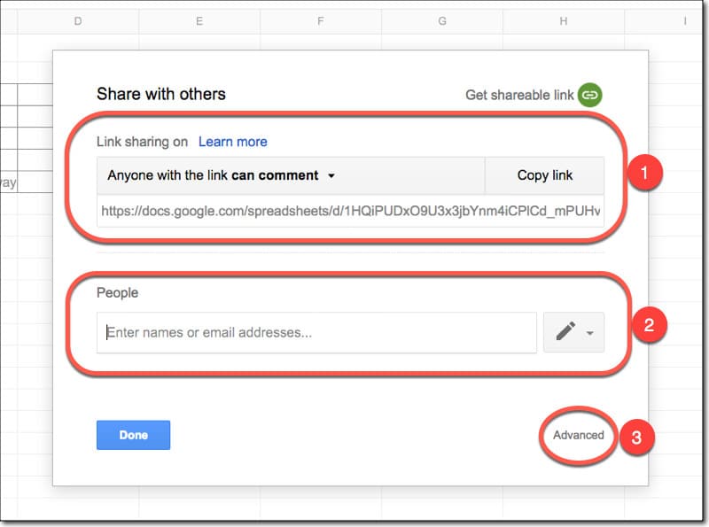
The Sharing options are found by clicking on the big blue button in the top right corner, which will open up the Sharing settings:
You can grab the link (the URL) to the Sheet, choose the share setting (view/comment/edit) and then share that link with people you want to see the Sheet. (1)
Or, you can enter someone’s email address directly, choose the share setting (view/comment/edit) and then share the Sheet directly with the person. (2)
If you want to review the sharing settings or have even more control, click the Advanced options buttons. (3)
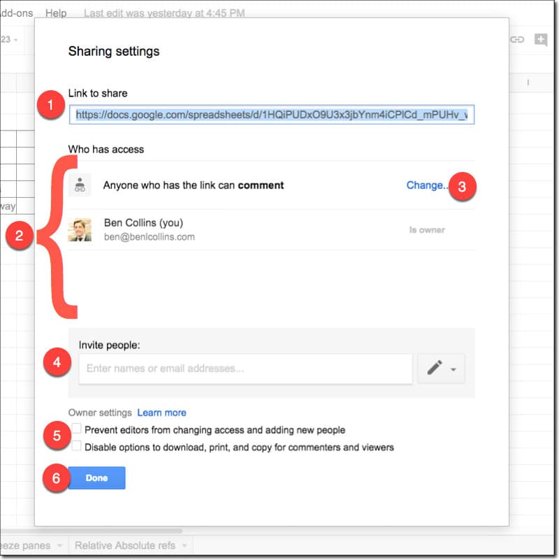
The Advanced sharing settings window:
Here you can:
> Grab the sharing link (1)
> Review who has access (2)
> Change the access rights of anyone listed (3)
> Invite new people to access the Sheet (4)
> Change the advanced owner settings, to restrict who can control the sharing settings and specific view/comment rights (5)
> Confirm when you’re finished (6)
I’ve used the link from the sharing settings to share the template for this tutorial with you!
Real-time Collaboration
Ok, so you’ve shared your Sheet with someone. If they open it whilst you’re still working in the Sheet you’ll see their cursor show up on whatever cell (or range) they’ve selected. It’ll be a different color, for example green to your blue.
If they enter data or delete data you’ll see it happening in real-time!
In this case my active cell is the blue-outlined cell. I see somebody else, denoted by the green-outlined cell, show up in this Sheet and enter data into a few cells before deleting it.
5. How to use Google Sheets: Intermediate techniques
Freeze panes
This is one of the most useful tricks you can learn in Google Sheets, which is why I’m recommending you learn it today.
Sooner or later you’ll work with a table of data that continues beyond the area you see on the screen (right now for example, I can see as far as row 26, but it depends on your screen size and other factors).
When you scroll down to look at data further down in your table, you lose the column headings off the top of your screen, and therefore can’t see the context of your columns.
Of course, scrolling up and down to see what the column headings are makes no sense. It’s a sure path to spreadsheet errors and insanity!
Have a look at this data table showing the tallest buildings in the world, which extends below the bottom of what you can see on a single screen in Sheets. Scrolling results in the heading row disappearing, so you no longer know which columns are which:
What you need to do is freeze the heading rows.
Thankfully it’s super easy.
Click on the row number of the row with your column headings in (e.g. row 3), then from the menu choose:
View > Freeze > Up to current row (3)
Now your headings will stay in place. Ah, that’s much better!
You can do the same with columns, if you wished to freeze names for example, so you can scroll horizontally across lots of columns of data.
Relative/Absolute references
This is arguably the hardest concept to grasp in this tutorial. If you understand it and can apply it, then you have a really good understanding of how spreadsheets work and you’re well on your way to being a skilled user.
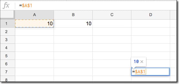
Suppose you have some data in cell A1 and you enter the following formula into cell B1:
= A1
This formula will retrieve whatever data is in cell A1 and show it in cell B1.
Now copy the formula (Cmd + C on a Mac, or Ctrl + C on a PC) and paste it (Cmd + V on a Mac, or Ctrl + V on a PC) somewhere else on your Sheet, for example cell D5.
Nothing will show up in D5. In fact you may be wondering whether your copy-paste worked. Have a look in the formula bar and you should now see this however:
= C5
The formula is there, but it points to a different cell, not A1, so does not show the data from A1.
But it still points to the cell that is ONE TO THE LEFT AND ON THE SAME ROW as the original formula.
Ah ha! Eureka!
The formula copied perfectly, keeping the same structure, pointing to the cell on the left.
This amazing property is called a relative reference, meaning it’s in relation to the cell where the formula is (e.g. one to the left).
That’s why you can drag formulas down columns and they’ll change automatically to calculate with data from their row.
Got that?
Now then, if you want to fix your formula (for example so it always point to cell A1) then you’ll want to use what’s called Absolute Referencing.
We lock the cell reference in the formula, so Google Sheets knows to not move the reference when the formula is moved.
The syntax uses a dollar sign, $, in front of the column reference and in front of the row reference to lock them each respectively, like so:
= $A$1
Now, wherever you copy this formula, the output will always point to cell A1 and return you the data from cell A1.
Note, you can just lock the column or just lock the row reference, and leave the other part as a relative reference, but that is beyond the scope of this tutorial.
Working with formulas across sheets
Sticking with the topic of referencing other cells for the moment, how does one go about linking to data on a different Sheet?
Returning once again to our basic gym membership table for dead famous authors, in Sheet 1, let’s retrieve the table heading and print it out in Sheet 2 with this formula, entered into cell A1 on Sheet 2:
= Sheet1!A1
Note the exclamation point at the end of the reference to Sheet1, i.e. Sheet1!
Now let’s do a simple sum of data on Sheet 1, but show our answer on Sheet 2.
In cell A3 in Sheet 2, enter the following formula:
= SUM( Sheet1!F4:F7 )
This will return the sum of the range of cells F4 to F7 in Sheet 1 and print out the answer in Sheet 2.
Basic conditional formatting
Conditional formatting is a powerful technique to apply different formats (for example background shading) to cells based on some conditions.
Let’s see an example of conditional formatting, that is, formatting based on variable conditions.
For example, in a financial model, you might show positive asset growth with a green font color and a light green background, whilst negative growth might be shown with red lettering on a light red background. This gives extra context to your numbers, and pre-attentive attributes (the colors) help to convey the message more efficiently.
Taking the plain copy of the membership table (hit Cmd + Z on a Mac, or Ctrl + Z on a PC to go back if you need), highlight the final column of the membership fee, then from the menu:
Format > Conditional formatting
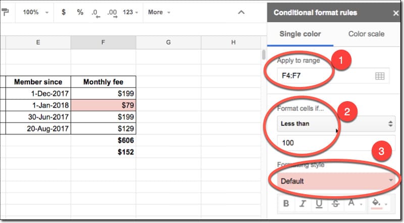
Here you can choose a rule, for example, values less than $100 and highlight them red:
Notice the range is shown (1), then a drop-down menu to choose a rule (2) and then the formatting option (3), which is default red in this case, although you can go completely custom if you choose.
The power of conditional formatting is to highlight data dynamically. The formatting is based on a rule, so if another value should drop below the threshold ($100 in this case), it will trigger the formatting rule and be highlighted red.
Sorting your data is a common request, for example to show transactions from highest revenue to lowest revenue, or customers with the greatest number to least number of purchases. Or to show suppliers in alphabetical order. You get the idea.
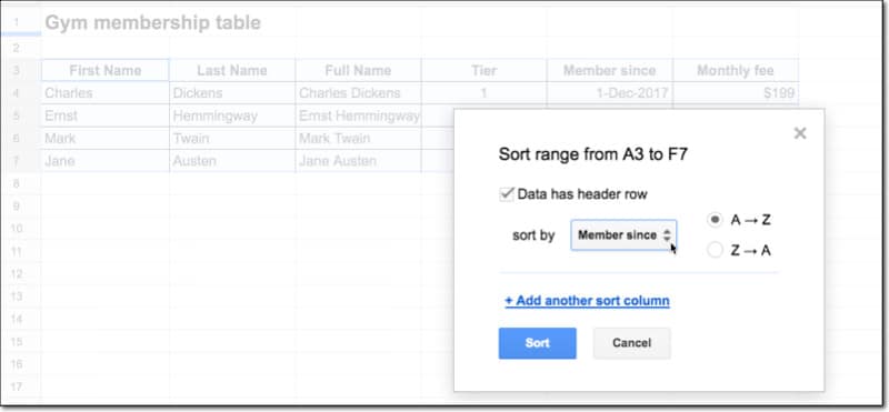
So let’s sort the dead famous authors gym membership table, from earliest members to most recent members, i.e. we’ll sort our table based on the date column.
Highlight the whole table, including the header row. Then from the menu:
Data > Sort range…
and be sure to check the “Data has header row” option. Then you can select the column you want to sort by, and sort option from A to Z, or Z to A.
This re-sorts the table, showing the earliest members first:
Filtering data
The next step after sorting your data is to filter it to hide the stuff you don’t want to see. Then you can just look at the data that is relevant to the problem at hand.
Taking the world’s tallest buildings data again, let’s apply a filter to only show skyscrapers built before the 2000s.
Click somewhere inside the data table (click on a cell containing data in the table), and then add the filters from the menu:
Data > Filter
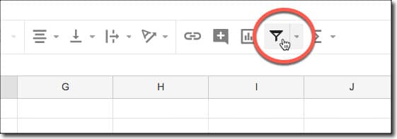
or by clicking this icon on the menu bar above your Sheet:
You’ll notice a light green shading applied to row and column headings of your filtered table, and also a green border around your table. Most importantly though, you’ll now have little green filter buttons in each of your heading cells.
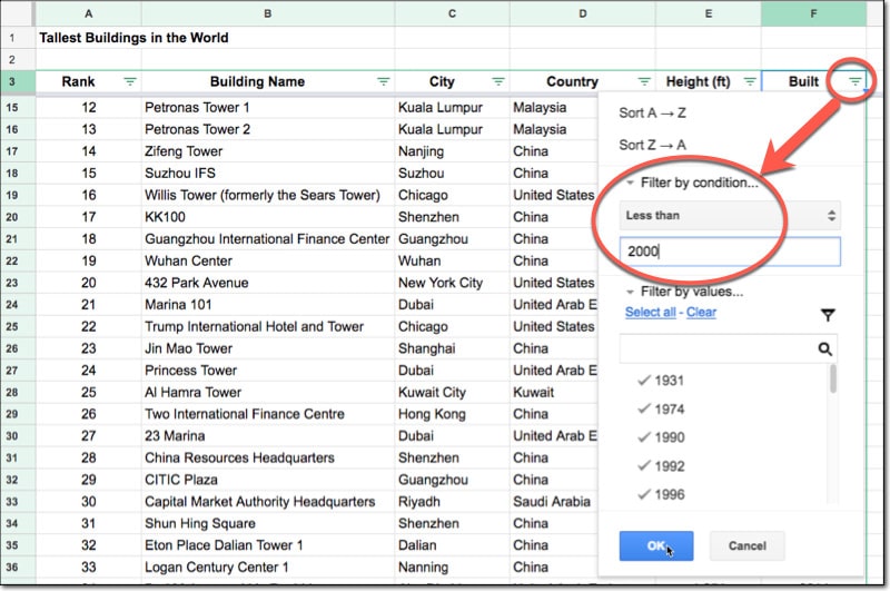
To filter out all the buildings built in the year 2000 or after, click the little green triangle next to the column heading Built, to bring up the filter menu.
You’ll notice you can manually select or de-select items to show. Let’s create a rule this time though.
Under the “Filter by condition” section, choose “Less than” and enter 2000 into the value box:
Hit OK.
Ta-da!
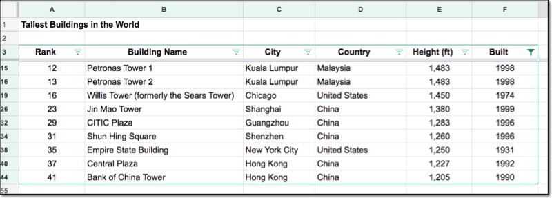
You’ll see a reduced table with just 9 results. The 9 skyscrapers built before the year 2000:
To remove the filter, click the green triangle button again (now solid green) and under the “Filter by conditions” set the rule to “None”.
There’s also a native FILTER function, by which you can formulaically filter your data.
As a final exercise with the tallest building data, let’s draw a chart to show the buildings built by year, so we can see the trend graphically.
First, let’s sort the table by the year Built column, from oldest to newest. We can do this using the sort function that is provided in the menu when you click on the green triangle (from the filter).
Then highlight this single column called Built and from the menu:
Insert > Chart
This creates a default chart in your window and opens the chart editing tool in a sidebar.
Here you can change your data range and chart type, as well as a multitude of chart custom formatting options (which are also generally accessible by clicking on the elements directly in the chart).
A chart is an object in your Sheet now. Click it to select it, so it has a blue border around it. You can resize it and drag it to move it, just as you would with an image.
Using the Explore feature
The robots are coming!
Soon we won’t have to create complex formulas or charts ourselves. We’ll simply ask our Sheet to do it for us. Sound far-fetched?
Well, you can do that now! The future is here.
(Soon we won’t have to open Google Sheets at all, we’ll simply type, or more likely speak, our data questions into a dashboard console, and out will pop the answers, but I digress.)
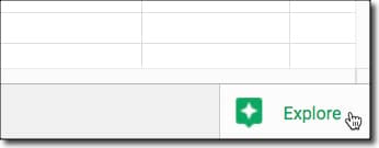
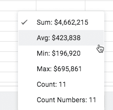
Google Sheets has a feature called Explore, powered by Machine Learning/AI/Deep Learning/Neural Network sorcery, that will ingest your data, analyze it and show you some common answers (like the SUM, COUNTs etc. we’ve seen so far) and basic charts:
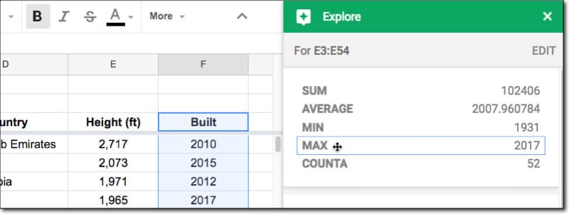
Let’s see an example, using the data about the world’s tallest buildings. Highlighting the column showing the years when each skyscraper was built and then clicking on the Explore button (bottom right corner) leads to these insights:
52 buildings in my set. The earliest tower on the list was built in 1931 (the venerable Empire State Building!) and the most recent was built in 2017. The average of all the years built is 2007.
Some interesting and useful data points, without having to do a lick of work!
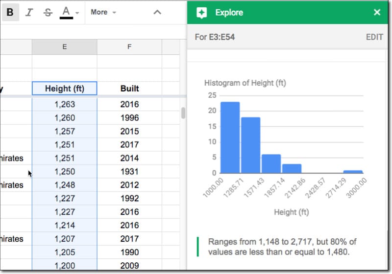
I mentioned charts, so let’s see an example of that with the Height (ft) column. Google Sheets Explore creates a Histogram for us, showing the distribution of tower heights:
We also get this interesting and insightful summary:
“Ranges from 1,148 to 2,717, but 80% of values are less than or equal to 1,480.”
Wow! At a glance, we have the min and max heights, but more impressive, we know that 80% are under 1,480ft tall.
Not all of the “insights” are useful, and I don’t use this feature much myself yet, but it shows a glimpse of how we’ll all work with Sheets in the future.
If you’re still not worried about AI taking over your job (whether that’s data analysis work or something else) in the next 10 to 50 years, then have a read of this article.
BONUS: VLOOKUP
No “How to use Google Sheets” article would be complete without at least a quick look at the VLOOKUP function.
Why?
Because it’s the most famous function. Tell anyone you work with data and spreadsheets and they’ll immediately ask, “yes, but do you know how to do a VLOOKUP?”
It’s a good bellwether for spreadsheet competency, even though there are ultimately better ways to work with data. It’s also a relatively advanced formula compared to what we’ve seen so far, so if you can understand it, it bodes well.
What does it do then?
It’s used to search for a term and return information about that term from a different table.
Generally, it’s used when you have two tables that share some common attribute (e.g. a name, ID number, or email), but otherwise, store different information. Suppose you want to bring this information together though. Well, you can, and you link the information via that common attribute.
One table might have details an employee’s name and address, and the other table might have their name and work details like title and salary. You can use the VLOOKUP function to bring these bits of data together in a single table.
In words: you select a search term that you search for in the first column of the search table. If you find it, you return a piece of information from the search table that relates to the search term (because it’s on the same row). The column number refers to which column of the search table you return the data from (1 being the column you searched in, so typically this number is 2 or greater).
Let’s see an example, by adding addresses to the dead famous authors’ gym membership table.
I’ve added a second table to Sheet 1, showing the addresses of our dead famous authors. What I’d like to do is add that data to the original gym table.
I want to do it efficiently with the VLOOKUP formula, rather than adding them manually. Not only is it much, much faster with larger tables (imagine ten thousand rows of data), but it’s also less error-prone.
The address table is in columns I and J, with the names in column I and addresses in column J.
So I’ll search for my author name in column I and return the address from column J, and print the output into whichever cell I created my formula in.
The formula is:
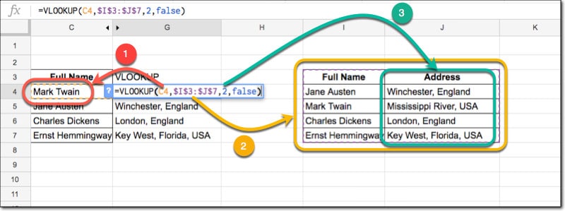
= VLOOKUP( C4, $I$3:$J$7, 2, FALSE )
And this is what’s happening:
I search for the name (1) in the search table (2) and return the data from column 2 of the search table (3).
I don’t expect you to understand all of this immediately (and there’s a lot more to this formula than what I’ve shown here), but if you try it out and persevere, you’ll get there and realize it’s actually not too difficult.
(The FALSE argument, the final piece of information in the VLOOKUP formula means you want to do an exact match. 99.9% of the time you use a VLOOKUP, you’ll want to use FALSE.)
💡 Learn more Check out my brand new beginner’s course: Google Sheets Essentials. This is a 100% online, on-demand video training course designed specifically to help you boost your spreadsheet skills.
The old adage “Practice makes perfect” is as true for Google Sheets as anything else, so hop to it!
Keep up-to-date with new articles, course launches and exclusive offers, by signing up for my Google Sheets newsletter, and get my free Google Sheets ebook with 100 tips.
 💡 Learn moreLearn how to write Apps Script and turbocharge your Google Workspace experience with the new Beginner Apps Script course
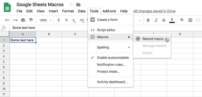


 1. How to use Google Sheets