Google announced Named Functions and 9 other new functions on 24th August 2022.
The biggest news here is the new feature called Named Functions. Named Functions let you save and name your own custom formulas, built with regular Sheets functions, and then re-use them in other Google Sheet files. It’s a HUGE step toward making formulas reusable.
Let’s look at the named functions and the 9 new functions:
- Named Functions
- LAMBDA Function
- MAP Function
- REDUCE Function
- MAKEARRAY Function
- SCAN Function
- BYROW Function
- BYCOL Function
- XLOOKUP Function
- XMATCH Function
1. Named Functions
Named Functions in Google Sheets let you save and name your own custom formulas, using all the built-in functions.
That complex financial formula you created… sure, turn it into a named function called =BENFINANCE(input1,input2,…) and use that instead!
And best of all, you can re-use these named functions in other Google Sheet files.
Here’s an example of a named function I created, called STARCHART, that draws mini star rating charts and can be reused in other Sheets:
Learn more about Named Functions
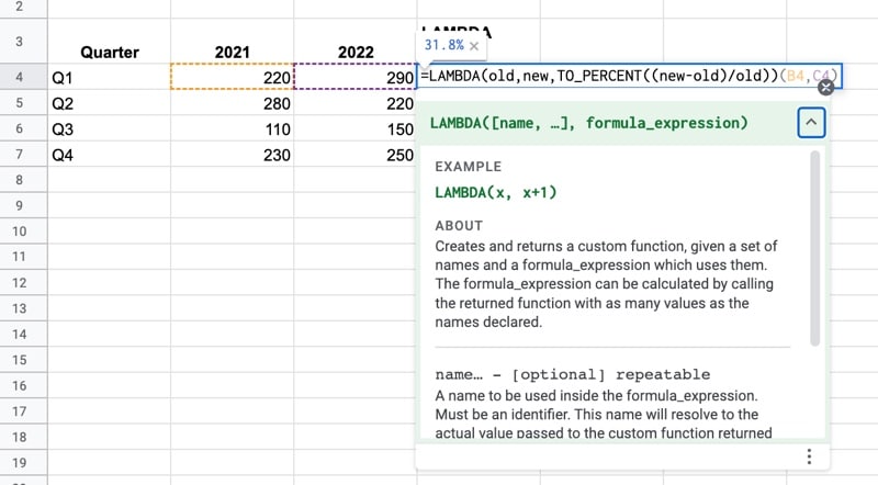
2. LAMBDA Function
The LAMBDA function in Google Sheets creates a custom function with placeholder inputs, instead of the usual A1 type cell or range references.
The main use case for the LAMBDA function is to work with other new lambda helper functions, like MAP, REDUCE, SCAN, MAKEARRAY, BYCOL, and BYROW.
LAMBDA functions are also the underlying technology for Named Functions, which we saw above.
Here’s an example LAMBDA function to calculate percent change:
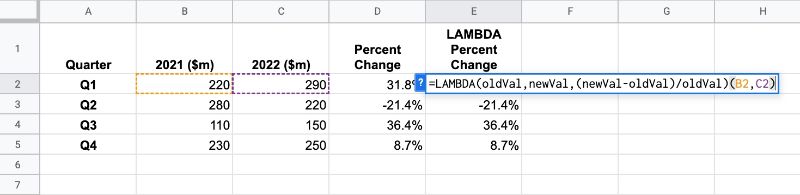
In this case though, you’d be better off creating a named function called PERCENTCHANGE rather than creating this lambda function explicitly.
Learn more about the LAMBDA function
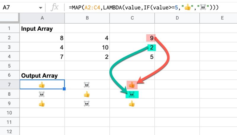
3. MAP Function
The MAP function in Google Sheets creates an array of data from an input range, where each value is “mapped” to a new value based on a custom LAMBDA function.
It’s the same idea as the MAP function in programming, a way to loop over an array of data and do something with each element of the array.
I think this formula is going to be super useful!
Here’s how the MAP function works, showing a silly transformation of values into emojis using an IF function as the lambda expression:
Learn more about the MAP Function
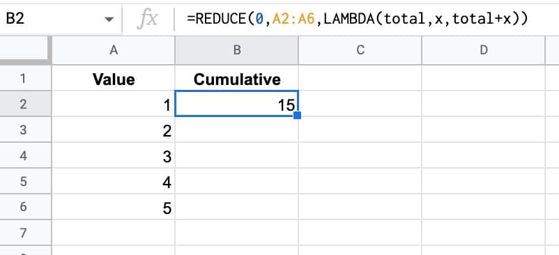
4. REDUCE Function
The REDUCE function in Google Sheets operates on an array (like the MAP function). It turns that array input into a single accumulated value, by applying a custom LAMBDA function to each element of the array. I.e. it reduces an array down to a single value.
For example, this simple REDUCE function calculates a cumulative total (yes, using the SUM function is easier, but this reduce example is just for illustration):
Learn more about the REDUCE Function
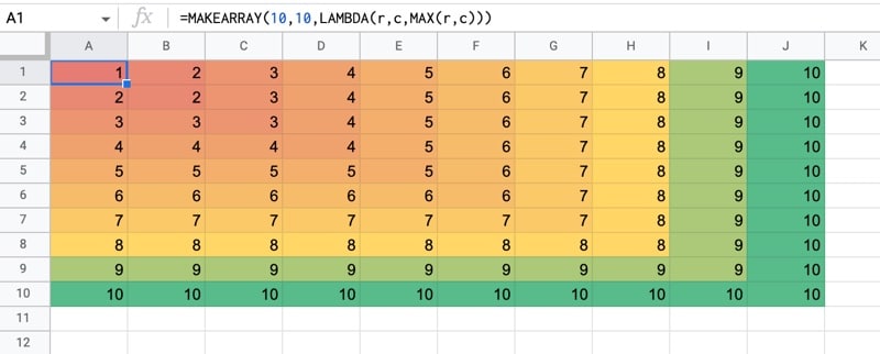
5. MAKEARRAY Function
The MAKEARRAY function in Google Sheets generates an array of a specified size, with each value calculated by a custom lambda function.
It’s like the SEQUENCE or RANDARRAY functions, except that in this case a lambda function is applied to each value in the array, so you can generate more complex arrays.
The lamba function has access to the row and column indices for each value.
Here the lambda evaluates the max of the row and column indices and then I added a heat map to that.
Learn more about the MAKEARRAY function
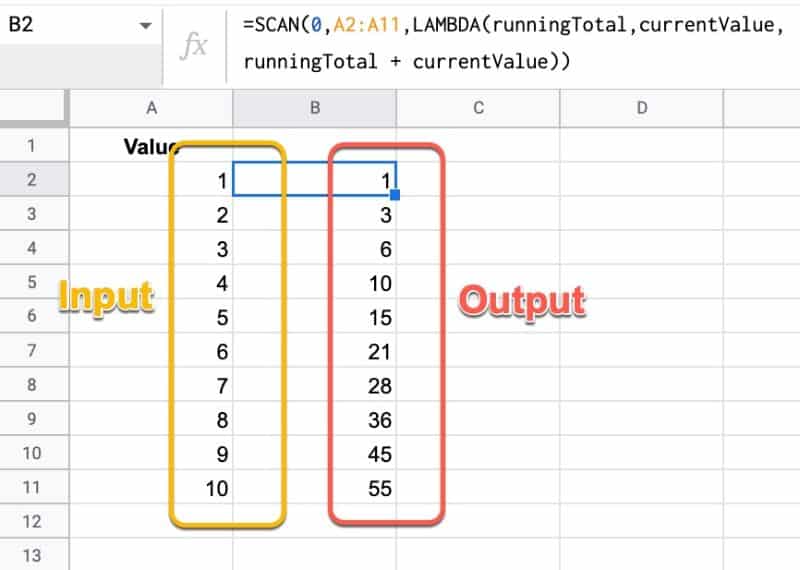
6. SCAN Function
The SCAN function in Google Sheets scans an array by applying a LAMBDA function to each value, moving row by row. The output is an array of intermediate values obtained at each step.
The most obvious application to create running totals of your data, like so:
Learn more about the SCAN Function
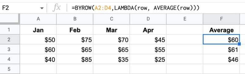
7. BYROW Function
The BYROW function in Google Sheets operates on an array or range and returns a new column array, created by grouping each row to a single value.
The value for each row is obtained by applying a lambda function on that row.
For example, we can use a single BYROW formula to calculate the average score of all three rows in the input array:
Learn more about the BYROW function
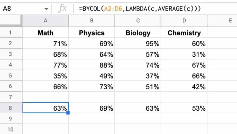
8. BYCOL Function
The BYCOL function operates in the same way as the BYROW function, but groups each column to a single value and returns a new row array.
In this example, the BYCOL formula outputs a row of average values:
Learn more about the BYCOL function
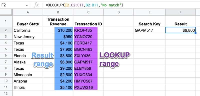
9. XLOOKUP Function
Yes! We have the awesome XLOOKUP function in Google Sheets now!!
It’s a more powerful and flexible version of the VLOOKUP function. It shares some similar capabilities to the INDEX/MATCH combination formulas.
XLOOKUP can lookup to the left, from the bottom up, and even use binary search if you’re working with really large datasets.
Here’s an example of the XLOOKUP performing a leftward lookup:
Learn more about the XLOOKUP Function
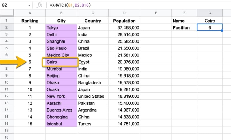
10. XMATCH Function
Last but not least is the XMATCH function, a more powerful and flexible version of the MATCH function.
It has more matching modes and search options than the plain MATCH function.
Here’s a simple XMATCH example:
Learn more about the XMATCH Function
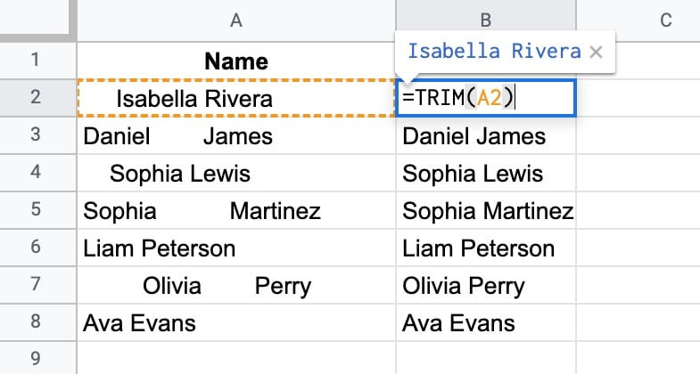
 💡 Learn more