The VLOOKUP function in Google Sheets is a vertical lookup function. You use it to search for an item in a column and return data from that row if a match is found.
In the following example, we use a VLOOKUP formula to search for “Charles Dickens” in column 1. When we find it, the formula returns the value from the 4th column of the lookup table to give a result of $299.
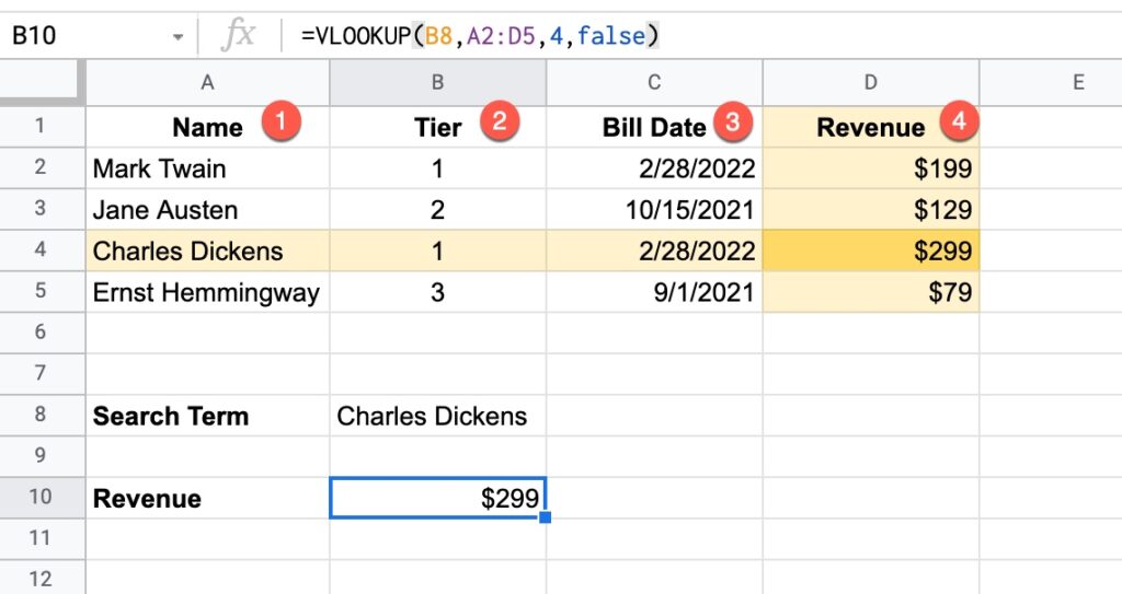
In this example, the VLOOKUP function is:
=VLOOKUP(B8,A2:D5,4,false)Let’s break this formula down:
B8 is the search term: “Charles Dickens”
The VLOOKUP looks down the first column of the lookup table: A2:D5
If it finds the search term, it then looks across that row to the column indicated by the Index number: 4
It then returns the value from column 4 as the answer, which is $299 in this example.
The final argument is false, meaning this is an exact match.
VLOOKUP can also handle approximate matching as well as wildcard searches. These more advanced use cases are explored further below.
Continue reading VLOOKUP Function in Google Sheets: The Essential Guide